cover

作者: Nikhil Buduma 
出版社: O'Reilly Media
副标题: Designing Next-Generation Machine Intelligence Algorithms
出版年: 2017-6-29
页数: 304
定价: USD 43.99
装帧: Paperback
ISBN: 9781491925614

Chapter 1. The Neural Network
Chapter 2. Training Feed-Forward Neural Networks
Chapter 3. Implementing Neural Networks in TensorFlow
Chapter 4. Beyond Gradient Descent
Chapter 5. Convolutional Neural Networks
Chapter 6. Embedding and Representation Learning
Chapter 7. Models for Sequence Analysis
Chapter 8. Memory Augmented Neural Networks
Chapter 9. Deep Reinforcement Learning

Chapter 1. The Neural Network

The Neuron

1-6

Figure 1-6. A functional description of a biological neuron’s structure

The neuron receives its inputs along antennae-like structures called dendrites. Each of these incoming connections is dynamically strengthened or weakened based on how often it is used (this is how we learn new concepts!), and it’s the strength of each connection that determines the contribution of the input to the neuron’s output. After being weighted by the strength of their respective connections, the inputs are summed together in the cell body. This sum is then transformed into a new signal that’s propagated along the cell’s axon and sent off to other neurons.

1-7

Figure 1-7. Schematic for a neuron in an artificial neural net

Just as in biological neurons, our artificial neuron takes in some number of inputs, $x_1, x_2, \cdots, x_n$, each of which is multiplied by a specific weight, $w_1, w_2, \cdots, w_n$. These weighted inputs are, as before, summed together to produce the logit of the neuron, $z=\sum_{i=0}^n w_ix_i$. In many cases, the logit also includes a bias, which is a constant (not shown in the figure). The logit is then passed through a function to produce the output . This output can be transmitted to other neurons.

Let’s reformulate the inputs as a vector $x = [x_1,x_2,\cdots,x_n]$ and the weights of the neuron as $w = [w_1,w_2,\cdots,w_n]$. Then we can re-express the output of the neuron as $y=f(x \cdot w + b)$, where b is the bias term.

Feed-Forward Neural Networks

1-9

Figure 1-9. A simple example of a feed-forward neural network with three layers (input, one hidden, and output) and three neurons per layer

The bottom layer of the network pulls in the input data. The top layer of neurons (output nodes) computes our final answer. The middle layer(s) of neurons are called the hidden layers, and we let $w_{i,j}^{(k)}$ be the weight of the connection between the $i^{th}$ neuron in the $k^{th}$ layer with the $j^{th}$ neuron in the ${k+1}^{st}$ layer. These weights constitute our parameter vector, $\theta$, our ability to solve problems with neural networks depends on finding the optimal values to plug into $\theta$.

We note that in this example, connections only traverse from a lower layer to a higher layer. There are no connections between neurons in the same layer, and there are no connections that transmit data from a higher layer to a lower layer. These neural networks are called feed-forward networks.

Linear Neurons

1-10

Figure 1-10. An example of a linear neuron

Sigmoid, Tanh, and ReLU Neurons

Sigmoid

$f(z)=\frac{1}{1+e^{-z}}$

1-11

Figure 1-11. The output of a sigmoid neuron as z varies

Tanh

Tanh neurons use a similar kind of S-shaped nonlinearity, but instead of ranging from 0 to 1, the output of tanh neurons range from −1 to 1.

1-12

Figure 1-12. The output of a tanh neuron as z varies

ReLU

Restricted linear unit (ReLU) neuron uses the function f(z)=max(0,z), resulting in a characteristic hockey-stick-shaped response, as shown in Figure 1-13.

1-13

Figure 1-13. The output of a ReLU neuron as z varies

Softmax Output Layers

We require the sum of all the outputs to be equal to 1. Letting $z_i$ be the logit of the $i^{th}$ softmax neuron, we can achieve this normalization by setting its output to:

$y_i=\frac{e^{z_i}}{\sum_i e^{z_j}}$

Chapter 2. Training Feed-Forward Neural Networks

The Fast-Food Problem

2-1

Figure 2-1. This is the neuron we want to train for the fast-food problem

In this case, let’s say we want to minimize the square error over all of the training examples that we encounter. More formally, if we know that $t^{(i)}$ is the true answer for the $i^{th}$ training example and $y^{(i)}$ is the value computed by the neural network, we want to minimize the value of the error function E:

$E=\frac{1}{2}\sum_i(t^{(i)}-y^{(i)})^2$

Gradient Descent

Let’s say our linear neuron only has two inputs(and thus only two weights, $w_1$ and $w_2$). Then we can imagine a three-dimensional space where the horizontal dimensions correspond to the weights $w_1$ and $w_2$, and the vertical dimension corresponds to the value of the error function E.

2-2

Figure 2-2. The quadratic error surface for a linear neuron

We can also conveniently visualize this surface as a set of elliptical contours, where the minimum error is at the center of the ellipses.

In fact, it turns out that the direction of the steepest descent is always perpendicular to the contours. This direction is expressed as a vector known as the gradient.

Suppose we randomly initialize the weights of our network so we find ourselves somewhere on the horizontal plane. By evaluating the gradient at our current position, we can find the direction of steepest descent, and we can take a step in that direction. Then we’ll find ourselves at a new position that’s closer to the minimum than we were before. We can reevaluate the direction of steepest descent by taking the gradient at this new position and taking a step in this new direction. This algorithm is known as gradient descent.

2-3

Figure 2-3. Visualizing the error surface as a set of contours

The Delta Rule and Learning Rates

2-4

Figure 2-4. Convergence is difficult when our learning rate is too large

Define the learning rate $\epsilon$, we want:

\[\Delta w_k=-\epsilon \frac{\partial E}{\partial w_k}=-\epsilon\frac{\partial}{\partial w_k}(\frac{1}{2}\sum_i(t^{(i)}-y^{(i)})^2)=\sum_i \epsilon(t^{(i)}-y^{(i)})\frac{\partial y_i}{\partial w_k}=\sum_i \epsilon x_k^{(i)}(t^{(i)}-y^{(i)})\]

Gradient Descent with Sigmoidal Neurons

$z=\sum_k w_k x_k$

$y=\frac{1}{1+e^{-z}}$

Taking the derivative of the logit with respect to the inputs and the weights:

$\frac{\partial z}{\partial w_k}=x_k$

$\frac{\partial z}{\partial x_k}=w_k$

The derivative of the output with respect to the logit:

$\frac{dy}{dz}=\frac{e^{-z}}{(1+e^{-z})^2}=\frac{1}{1+e^{-z}}\frac{e^{-z}}{1+e^{-z}}=\frac{1}{1+e^{-z}}(1-\frac{1}{1+e^{-z}})=y(1-y)$

We then use the chain rule to get the derivative of the output with respect to each weight:

$\frac{\partial y}{\partial w_k}=\frac{dy}{dz}\frac{\partial z}{\partial w_k}=x_k y(1-y)$

Putting all of this together:

$\frac{\partial E}{\partial w_k}=\sum_i\frac{\partial E}{\partial y^{(i)}}\frac{\partial y^{(i)}}{\partial w_k}=-\sum_i x_k^{(i)} y^{(i)}(1-y^{(i)})(t^{(i)}-y^{(i)})$

Thus, the final rule for modifying the weights becomes:

$\Delta w_k=\sum_i \epsilon x_k^{(i)}y^{(i)}(1-y^{(i)})(t^{(i)}-y^{(i)})$

The Backpropagation Algorithm

2-5

Figure 2-5. Reference diagram for the derivation of the backpropagation algorithm

y:refer to the activity of a neuron
z:refer to the logit of the neuron

Calculate the error function derivatives at the output layer:

$E=\frac{1}{2}\sum_{j \in output}(t_j-y_j)^2 \Rightarrow \frac{\partial E}{\partial y_j}=-(t_j-y_j)$

Let’s presume we have the error derivatives for layer j. We now aim to calculate the error derivatives for the layer below it, layer i. To do so, we must accumulate information about how the output of a neuron in layer i affects the logits of every neuron in layer j. This can be done as follows, using the fact that the partial derivative of the logit with respect to the incoming output data from the layer beneath is merely the weight of the connection $w_{ij}$:

$\frac{\partial E}{\partial y_i}=\sum_j\frac{\partial E}{\partial z_j}\frac{d z_j}{d y_j}=\sum_j w_{ij}\frac{\partial E}{\partial z_j}$

$\frac{\partial E}{\partial z_j}=\frac{\partial E}{\partial y_j}\frac{d y_j}{d z_j}=y_j (1-y_j) \frac{\partial E}{\partial y_i}$

Combining these two together, we can finally express the error derivatives of layer i in terms of the error derivatives of layer j:

$\frac{\partial E}{\partial y_i}=\sum_j w_{ij}y_j(1-y_j)\frac{\partial E}{\partial y_j}$

$\frac{\partial E}{\partial w_{ij}}=\frac{\partial z_j}{\partial w_{ij}}\frac{\partial E}{\partial z_j}=y_i y_j(1-y_j)\frac{\partial E}{\partial y_j}$

Finally, we sum up the partial derivatives over all the training examples in our dataset.

$\Delta w_{ij}=-\sum_{k \in dataset} \epsilon y_i^{(k)}y_j^{(k)}(1-y_j^{(k)})\frac{\partial E^{(k)}}{\partial y_j^{(k)}}$

Stochastic and Minibatch Gradient Descent

2-6

Figure 2-6. Batch gradient descent is sensitive to saddle points, which can lead to premature convergence

SGD:

2-7

Figure 2-7. The stochastic error surface fluctuates with respect to the batch error surface, enabling saddle point avoidance

In mini-batch gradient descent, at every iteration, we compute the error surface with respect to some subset of the total dataset (instead of just a single example). This subset is called a minibatch, and in addition to the learning rate, minibatch size is another hyperparameter.

$\Delta w_{ij}=-\sum_{k \in minibatch} \epsilon y_i^{(k)}y_j^{(k)}(1-y_j^{(k)})\frac{\partial E^{(k)}}{\partial y_j^{(k)}}$

Test Sets, Validation Sets, and Overfitting

2-8

Figure 2-8. Two potential models that might describe our dataset: a linear model versus a degree 12 polynomial

2-9

Figure 2-9. Evaluating our model on new data indicates that the linear fit is a much better model than the degree 12 polynomial

2-10

Figure 2-10. A visualization of neural networks with 3, 6, and 20 neurons (in that order) in their hidden layer

2-11

Figure 2-11. A visualization of neural networks with one, two, and four hidden layers (in that order) of three neurons each

This leads to three major observations.First, the machine learning engineer is always working with a direct trade-off between overfitting and model complexity.

Second, it is very misleading to evaluate a model using the data we used to train it

2-12

Figure 2-12. We often split our data into nonoverlapping training and test sets in order to fairly evaluate our model

Third, it’s quite likely that while we’re training our data, there’s a point in time where instead of learning useful features, we start overfitting to the training set. To avoid that, we want to be able to stop the training process as soon as we start overfitting, to prevent poor generalization. To do this, we divide our training process into epochs. An epoch is a single iteration over the entire training set.

At the end of each epoch, we want to measure how well our model is generalizing. To do this, we use an additional validation set.

2-13

Figure 2-13. In deep learning we often include a validation set to prevent overfitting during the training process

2-14

Figure 2-14. Detailed workflow for training and evaluating a deep learning model

Preventing Overfitting in Deep Neural Networks

Regularization modifies the objective function that we minimize by adding additional terms that penalize large weights. In other words, we change the objective function so that it becomes $Error + \lambda f(\theta)$, where $f(\theta)$ grows larger as the components of $\theta$ grow larger, and $\lambda$ is the regularization strength (another hyperparameter).

The most common type of regularization in machine learning is L2 regularization. It can be implemented by augmenting the error function with the squared magnitude of all weights in the neural network. In other words, for every weight w in the neural network, we add $\frac{1}{2}\lambda w^2$ to the error function. The L2 regularization has the intuitive interpretation of heavily penalizing peaky weight vectors and preferring diffuse weight vectors. This has the appealing property of encouraging the network to use all of its inputs a little rather than using only some of its inputs a lot. Of particular note is that during the gradient descent update, using the L2 regularization ultimately means that every weight is decayed linearly to zero. Because of this phenomenon, L2 regularization is also commonly referred to as weight decay.

2-15

Figure 2-15. A visualization of neural networks trained with regularization strengths of 0.01, 0.1, and 1 (in that order)

Another common type of regularization is L1 regularization. Here, we add the term $\lambda w $ for every weight w in the neural network. The L1 regularization has the intriguing property that it leads the weight vectors to become sparse during optimization (i.e., very close to exactly zero). In other words, neurons with L1 regularization end up using only a small subset of their most important inputs and become quite resistant to noise in the inputs. In comparison, weight vectors from L2 regularization are usually diffuse, small numbers. L1 regularization is very useful when you want to understand exactly which features are contributing to a decision. If this level of feature analysis isn’t necessary, we prefer to use L2 regularization because it empirically performs better.

Max norm constraints enforce an absolute upper bound on the magnitude of the incoming weight vector for every neuron and use projected gradient descent to enforce the constraint. In other words, any time a gradient descent step moves the incoming weight vector such that $\lVert w \rVert^2 > c$, we project the vector back onto the ball (centered at the origin) with radius c.

While training, dropout is implemented by only keeping a neuron active with some probability p (a hyperparameter), or setting it to zero otherwise. Intuitively, this forces the network to be accurate even in the absence of certain information. It prevents the network from becoming too dependent on any one (or any small combination) of neurons. Expressed more mathematically, it prevents overfitting by providing a way of approximately combining exponentially many different neural network architectures efficiently.

2-16

Figure 2-16. Dropout sets each neuron in the network as inactive with some random probability during each minibatch of training

Chapter 3. Implementing Neural Networks in TensorFlow

Installing TensorFlow

import tensorflow as tf
deep_learning = tf.constant('Deep Learning')
session = tf.Session()
session.run(deep_learning)

'Deep Learning'

a = tf.constant(2)
b = tf.constant(3)
multiply = tf.multiply(a, b)
session.run(multiply)

6

According to the tensorflow 1.0.0 release notes

tf.mul, tf.sub and tf.neg are deprecated in favor of tf.multiply, tf.subtract and tf.negative.

Creating and Manipulating TensorFlow Variables

# Common tensors from the TensorFlow API docs

tf.zeros(shape, dtype=tf.float32, name=None)
tf.ones(shape, dtype=tf.float32, name=None)
tf.random_normal(shape, mean=0.0, stddev=1.0, 
                 dtype=tf.float32, seed=None, 
                 name=None)
tf.truncated_normal(shape, mean=0.0, stddev=1.0, 
                    dtype=tf.float32, seed=None, 
                    name=None)
tf.random_uniform(shape, minval=0, maxval=None, 
                  dtype=tf.float32, seed=None, 
                  name=None)

When we call tf.Variable, three operations are added to the computation graph:

The operation producing the tensor we use to initialize our variable
The tf.assign operation, which is responsible for filling the variable with the initializing tensor prior to the variable’s use
The variable operation, which holds the current value of the variable

3-1

Figure 3-1. Three operations are added to the graph when instantiating a TensorFlow variable. In this example, we instantiate the variable weights using a random normal initializer.

TensorFlow Operations

Table 3-1. A summary table of TensorFlow operations

Category	Examples
Element-wise mathematical operations	Add, Sub, Mul, Div, Exp, Log, Greater, Less, Equal, …
Array operations	Concat, Slice, Split, Constant, Rank, Shape, Shuffle, …
Matrix operations	MatMul, MatrixInverse, MatrixDeterminant, …
Stateful operations	Variable, Assign, AssignAdd, …
Neural network building blocks	SoftMax, Sigmoid, ReLU, Convolution2D, MaxPool, …
Checkpointing operations	Save, Restore
Queue and synchronization operations	Enqueue, Dequeue, MutexAcquire, MutexRelease, …
Control flow operations	Merge, Switch, Enter, Leave, NextIteration

Placeholder Tensors

A variable is insufficient because it is only meant to be initialized once. Just as variables need to be initialized the first time the computation graph is built, placeholders need to be filled every time the computation graph (or a subgraph) is run.

x = tf.placeholder(tf.float32, name="x", shape=[None, 784])
W = tf.Variable(tf.random_uniform([784,10], -1, 1), name="W")
multiply = tf.matmul(x, W)

define a placeholder where x represents a minibatch of data stored as float32’s
x has 784 columns
x has an undefined number of rows. This means that x can be initialized with an arbitrary number of data samples
W demension:784*10, range $\in$ [-1,1]

Sessions in TensorFlow

import tensorflow as tf
from read_data import get_minibatch()

x = tf.placeholder(tf.float32, name="x", shape=[None, 784])
W = tf.Variable(tf.random_uniform([784, 10], -1, 1), name="W")
b = tf.Variable(tf.zeros([10]), name="biases")
output = tf.matmul(x, W) + b

init_op = tf.global_variables_initializer()

sess = tf.Session() 
sess.run(init_op)
feed_dict = {"x" : get_minibatch()}
sess.run(output, feed_dict=feed_dict)

3-2

Figure 3-2. This is a an example of a simple computational graph in TensorFlow

def my_network(input):
    W_1 = tf.Variable(tf.random_uniform([784, 100], -1, 1), name="W_1")
    b_1 = tf.Variable(tf.zeros([100]), name="biases_1")
    output_1 = tf.matmul(input, W_1) + b_1

    W_2 = tf.Variable(tf.random_uniform([100, 50], -1, 1), name="W_2")
    b_2 = tf.Variable(tf.zeros([50]), name="biases_2")
    output_2 = tf.matmul(output_1, W_2) + b_2

    W_3 = tf.Variable(tf.random_uniform([50, 10], -1, 1), name="W_3")
    b_3 = tf.Variable(tf.zeros([10]), name="biases_3")
    output_3 = tf.matmul(output_2, W_3) + b_3

    # printing names
    print "Printing names of weight parameters"
    print W_1.name, W_2.name, W_3.name
    print "Printing names of bias parameters"
    print b_1.name, b_2.name, b_3.name

    return output_3

i_1 = tf.placeholder(tf.float32, [1000, 784], name="i_1")
my_network(i_1)

Printing names of weight parameters
W_1:0 W_2:0 W_3:0
Printing names of bias parameters
biases_1:0 biases_2:0 biases_3:0
<tf.Tensor 'add_2:0' shape=(1000, 10) dtype=float32>

i_2 = tf.placeholder(tf.float32, [1000, 784], name="i_2")
my_network(i_2)

Printing names of weight parameters
W_1_1:0 W_2_1:0 W_3_1:0
Printing names of bias parameters
biases_1_1:0 biases_2_1:0 biases_3_1:0
<tf.Tensor 'add_5:0' shape=(1000, 10) dtype=float32>

TensorFlow’s variable scoping mechanisms are largely controlled by two functions:

tf.get_variable(<name>, <shape>, <initializer>)
- Checks if a variable with this name exists, retrieves the variable if it does, or creates it using the shape and initializer if it doesn’t.
tf.variable_scope(<scope_name>)
- Manages the namespace and determines the scope in which tf.get_variable operates.

def layer(input, weight_shape, bias_shape):
    weight_init = tf.random_uniform_initializer(minval=-1, maxval=1)
    bias_init = tf.constant_initializer(value=0)
    W = tf.get_variable("W", weight_shape, initializer=weight_init)
    b = tf.get_variable("b", bias_shape, initializer=bias_init)
    return tf.matmul(input, W) + b

def my_network(input):
    with tf.variable_scope("layer_1"):
        output_1 = layer(input, [784, 100], [100])
     
    with tf.variable_scope("layer_2"):
        output_2 = layer(output_1, [100, 50], [50])
     
    with tf.variable_scope("layer_3"):
        output_3 = layer(output_2, [50, 10], [10])
     
    return output_3

Now let’s try to call my_network twice, just like we did in the preceding code block:

i_1 = tf.placeholder(tf.float32, [1000, 784], name="i_1")
my_network(i_1)

<tf.Tensor 'layer_3/add:0' shape=(1000, 10) dtype=float32>

i_2 = tf.placeholder(tf.float32, [1000, 784], name="i_2")
my_network(i_2)

---------------------------------------------------------------------------
ValueError                                Traceback (most recent call last)
<ipython-input-8-e22e9d54b2f8> in <module>()
      1 i_2 = tf.placeholder(tf.float32, [1000, 784], name="i_2")
----> 2 my_network(i_2)

<ipython-input-6-fd851d0f603b> in my_network(input)
      8 def my_network(input):
      9      with tf.variable_scope("layer_1"):
---> 10           output_1 = layer(input, [784, 100], [100])
     11 
     12      with tf.variable_scope("layer_2"):

<ipython-input-6-fd851d0f603b> in layer(input, weight_shape, bias_shape)
      2      weight_init = tf.random_uniform_initializer(minval=-1, maxval=1)
      3      bias_init = tf.constant_initializer(value=0)
----> 4      W = tf.get_variable("W", weight_shape, initializer=weight_init)
      5      b = tf.get_variable("b", bias_shape, initializer=bias_init)
      6      return tf.matmul(input, W) + b

/Users/zhangjun/anaconda/lib/python2.7/site-packages/tensorflow/python/ops/variable_scope.pyc in get_variable(name, shape, dtype, initializer, regularizer, trainable, collections, caching_device, partitioner, validate_shape, use_resource, custom_getter)
   1047       collections=collections, caching_device=caching_device,
   1048       partitioner=partitioner, validate_shape=validate_shape,
-> 1049       use_resource=use_resource, custom_getter=custom_getter)
   1050 get_variable_or_local_docstring = (
   1051     """%s

/Users/zhangjun/anaconda/lib/python2.7/site-packages/tensorflow/python/ops/variable_scope.pyc in get_variable(self, var_store, name, shape, dtype, initializer, regularizer, trainable, collections, caching_device, partitioner, validate_shape, use_resource, custom_getter)
    946           collections=collections, caching_device=caching_device,
    947           partitioner=partitioner, validate_shape=validate_shape,
--> 948           use_resource=use_resource, custom_getter=custom_getter)
    949 
    950   def _get_partitioned_variable(self,

/Users/zhangjun/anaconda/lib/python2.7/site-packages/tensorflow/python/ops/variable_scope.pyc in get_variable(self, name, shape, dtype, initializer, regularizer, reuse, trainable, collections, caching_device, partitioner, validate_shape, use_resource, custom_getter)
    354           reuse=reuse, trainable=trainable, collections=collections,
    355           caching_device=caching_device, partitioner=partitioner,
--> 356           validate_shape=validate_shape, use_resource=use_resource)
    357 
    358   def _get_partitioned_variable(

/Users/zhangjun/anaconda/lib/python2.7/site-packages/tensorflow/python/ops/variable_scope.pyc in _true_getter(name, shape, dtype, initializer, regularizer, reuse, trainable, collections, caching_device, partitioner, validate_shape, use_resource)
    339           trainable=trainable, collections=collections,
    340           caching_device=caching_device, validate_shape=validate_shape,
--> 341           use_resource=use_resource)
    342 
    343     if custom_getter is not None:

/Users/zhangjun/anaconda/lib/python2.7/site-packages/tensorflow/python/ops/variable_scope.pyc in _get_single_variable(self, name, shape, dtype, initializer, regularizer, partition_info, reuse, trainable, collections, caching_device, validate_shape, use_resource)
    651                          " Did you mean to set reuse=True in VarScope? "
    652                          "Originally defined at:\n\n%s" % (
--> 653                              name, "".join(traceback.format_list(tb))))
    654       found_var = self._vars[name]
    655       if not shape.is_compatible_with(found_var.get_shape()):

ValueError: Variable layer_1/W already exists, disallowed. Did you mean to set reuse=True in VarScope? Originally defined at:

  File "<ipython-input-6-fd851d0f603b>", line 4, in layer
    W = tf.get_variable("W", weight_shape, initializer=weight_init)
  File "<ipython-input-6-fd851d0f603b>", line 10, in my_network
    output_1 = layer(input, [784, 100], [100])
  File "<ipython-input-7-0155c84ecd17>", line 2, in <module>
    my_network(i_1)

By default, sharing is not allowed (just to be safe!), but if we want to enable sharing within a variable scope, we can say so explicitly:

with tf.variable_scope("shared_variables") as scope:
    i_1 = tf.placeholder(tf.float32, [1000, 784], name="i_1")
    my_network(i_1)
    scope.reuse_variables()
    i_2 = tf.placeholder(tf.float32, [1000, 784], name="i_2")
    my_network(i_2)

Managing Models over the CPU and GPU

Supported devices are represented by string IDs and normally consist of the following:

“/cpu:0”
- The CPU of our machine.
“/gpu:0”
- The first GPU of our machine, if it has one.
“/gpu:1”
- The second GPU of our machine, if it has one.

To inspect which devices are used by the computational graph, we can initialize our TensorFlow session with the log_device_placement set to True:

sess = tf.Session(config=tf.ConfigProto(log_device_placement=True))

If we desire to use a specific device, we may do so by using with tf.device to select the appropriate device. If the chosen device is not available, however, an error will be thrown. If we would like TensorFlow to find another available device if the chosen device does not exist, we can pass the allow_soft_placement flag to the session variable as follows:

with tf.device('/gpu:2'):
  a = tf.constant([1.0, 2.0, 3.0, 4.0], shape=[2, 2], name='a')
  b = tf.constant([1.0, 2.0], shape=[2, 1], name='b')
  c = tf.matmul(a, b)

sess = tf.Session(config=tf.ConfigProto(
      allow_soft_placement=True, log_device_placement=True))

sess.run(c)

The following code is an example of multi-GPU code[fig 3-3]:

c = []

for d in ['/gpu:0', '/gpu:1']:
  with tf.device(d):
    a = tf.constant([1.0, 2.0, 3.0, 4.0], shape=[2, 2], 
                      name='a')
    b = tf.constant([1.0, 2.0], shape=[2, 1], name='b')
    c.append(tf.matmul(a, b))

with tf.device('/cpu:0'):
  sum = tf.add_n(c)

sess = tf.Session(config=tf.ConfigProto(
                   log_device_placement=True))

sess.run(sum)

3-3

Figure 3-3. Building multi-GPU models in a tower-like fashion

Specifying the Logistic Regression Model in TensorFlow

Our model uses a matrix W representing the weights of the connections in the network, as well as a vector b corresponding to the biases to estimate whether an input x belongs to class i using the softmax expression we talked about earlier:

$p(y=i

x)=softmax_i(Wx+b)=\frac{e^{W_ix+b_i}}{\sum_j e^{W_jx+b_j}}$

3-4

Figure 3-4. Interpreting logistic regression as a primitive neural network

We’ll build the the logistic regression model in four phases:

inference: produces a probability distribution over the output classes given a minibatch
loss: computes the value of the error function (in this case, the cross-entropy loss)
training: responsible for computing the gradients of the model’s parameters and updating the model
evaluate: will determine the effectiveness of a model

def inference(x):
    init = tf.constant_initializer(value=0)
    W = tf.get_variable("W", [784, 10], initializer=init)
    b = tf.get_variable("b", [10], initializer=init)
    output = tf.nn.softmax(tf.matmul(x, W) + b)

    w_hist = tf.summary.histogram("weights", W)
    b_hist = tf.summary.histogram("biases", b)
    y_hist = tf.summary.histogram("output", output)

    return output

def loss(output, y):
    dot_product = y * tf.log(output)

    # Reduction along axis 0 collapses each column into a
    # single value, whereas reduction along axis 1 collapses  
    # each row into a single value. In general, reduction along  
    # axis i collapses the ith dimension of a tensor to size 1.
    xentropy = -tf.reduce_sum(dot_product, reduction_indices=1)
    
    loss = tf.reduce_mean(xentropy)
    return loss

def training(cost, global_step):
    tf.summary.scalar("cost", cost)
    optimizer = tf.train.GradientDescentOptimizer(learning_rate)
    train_op = optimizer.minimize(cost, global_step=global_step)
    return train_op

def evaluate(output, y):
    correct_prediction = tf.equal(tf.argmax(output, 1), tf.argmax(y, 1))
    accuracy = tf.reduce_mean(tf.cast(correct_prediction, tf.float32))
    tf.summary.scalar("validation error", (1.0 - accuracy))
    return accuracy

tf.constant_initializer 常量初始化函数。
tf.reduce_sum 求和，由于求和的对象是tensor，所以是沿着tensor的某些维度求和。
- reduction_indice 是指沿tensor的哪些维度求和。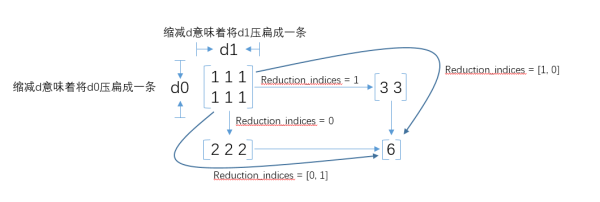
tf.equal 是对比这两个矩阵或者向量的相等的元素，如果是相等的那就返回True，反正返回False，返回的值的矩阵维度和A是一样的。
- 下面例子代码输出：[[ True True True False False]]

import tensorflow as tf
import numpy as np

A = [[1,3,4,5,6]]
B = [[1,3,4,3,2]]

with tf.Session() as sess:
    print(sess.run(tf.equal(A, B)))

tf.summary.scalar and tf.summary.histogram commands to log the cost for each minibatch, validation error, and the distribution of parameters

Logging and Training the Logistic Regression Model

import input_data
mnist = input_data.read_data_sets("data/", one_hot=True)

# Parameters
learning_rate = 0.01
training_epochs = 60
batch_size = 100
display_step = 1

with tf.Graph().as_default():
    x = tf.placeholder("float", [None, 784]) # mnist data image of shape 28*28=784
    y = tf.placeholder("float", [None, 10]) # 0-9 digits recognition => 10 classes

    output = inference(x)
    cost = loss(output, y)
    global_step = tf.Variable(0, name='global_step', trainable=False)
    train_op = training(cost, global_step)
    eval_op = evaluate(output, y)
    summary_op = tf.summary.merge_all()
    saver = tf.train.Saver()

    sess = tf.Session()
    summary_writer = tf.summary.FileWriter("logistic_logs/", graph=sess.graph)
    init_op = tf.global_variables_initializer()
    sess.run(init_op)

    # Training cycle
    for epoch in range(training_epochs):
        avg_cost = 0.
        total_batch = int(mnist.train.num_examples/batch_size)
        # Loop over all batches
        for i in range(total_batch):
            minibatch_x, minibatch_y = mnist.train.next_batch(batch_size)
            # Fit training using batch data
            sess.run(train_op, feed_dict={x: minibatch_x, y: minibatch_y})
            # Compute average loss
            avg_cost += sess.run(cost, feed_dict={x: minibatch_x, y: minibatch_y})/total_batch
        # Display logs per epoch step
        if epoch % display_step == 0:
            print "Epoch:", '%04d' % (epoch+1), "cost =", "{:.9f}".format(avg_cost)

            accuracy = sess.run(eval_op, feed_dict={x: mnist.validation.images, y: mnist.validation.labels})

            print "Validation Error:", (1 - accuracy)

            summary_str = sess.run(summary_op, feed_dict={x: minibatch_x, y: minibatch_y})
            summary_writer.add_summary(summary_str, sess.run(global_step))

            saver.save(sess, "logistic_logs/model-checkpoint", global_step=global_step)

print "Optimization Finished!"
accuracy = sess.run(eval_op, feed_dict={x: mnist.test.images, y: mnist.test.labels})
print "Test Accuracy:", accuracy

Extracting data/train-images-idx3-ubyte.gz
Extracting data/train-labels-idx1-ubyte.gz
Extracting data/t10k-images-idx3-ubyte.gz
Extracting data/t10k-labels-idx1-ubyte.gz
INFO:tensorflow:Summary name validation error is illegal; using validation_error instead.
Epoch: 0001 cost = 1.174406662
Validation Error: 0.1507999897
Epoch: 0002 cost = 0.661975267
Validation Error: 0.127799987793
Epoch: 0003 cost = 0.550479775
Validation Error: 0.119799971581
Epoch: 0004 cost = 0.496666517
Validation Error: 0.114000022411
Epoch: 0005 cost = 0.463729115
Validation Error: 0.109600007534
Epoch: 0006 cost = 0.440869012
Validation Error: 0.106599986553
Epoch: 0007 cost = 0.423876265
Validation Error: 0.104600012302
Epoch: 0008 cost = 0.410587048
Validation Error: 0.102800011635
Epoch: 0009 cost = 0.399861779
Validation Error: 0.100000023842
Epoch: 0010 cost = 0.390921709
Validation Error: 0.0985999703407
Epoch: 0011 cost = 0.383350472
Validation Error: 0.0975999832153
Epoch: 0012 cost = 0.376742928
Validation Error: 0.0957999825478
Epoch: 0013 cost = 0.370986774
Validation Error: 0.0952000021935
Epoch: 0014 cost = 0.365939115
Validation Error: 0.093800008297
Epoch: 0015 cost = 0.361372554
Validation Error: 0.0917999744415
Epoch: 0016 cost = 0.357271555
Validation Error: 0.090399980545
Epoch: 0017 cost = 0.353570737
Validation Error: 0.0889999866486
Epoch: 0018 cost = 0.350133936
Validation Error: 0.0878000259399
Epoch: 0019 cost = 0.347030580
Validation Error: 0.0888000130653
Epoch: 0020 cost = 0.344142686
Validation Error: 0.0870000123978
Epoch: 0021 cost = 0.341469975
Validation Error: 0.087199985981
Epoch: 0022 cost = 0.338988112
Validation Error: 0.0866000056267
Epoch: 0023 cost = 0.336671517
Validation Error: 0.0860000252724
Epoch: 0024 cost = 0.334482374
Validation Error: 0.0852000117302
Epoch: 0025 cost = 0.332421122
Validation Error: 0.0856000185013
Epoch: 0026 cost = 0.330536905
Validation Error: 0.0856000185013
Epoch: 0027 cost = 0.328713858
Validation Error: 0.0849999785423
Epoch: 0028 cost = 0.327041571
Validation Error: 0.0849999785423
Epoch: 0029 cost = 0.325404955
Validation Error: 0.0845999717712
Epoch: 0030 cost = 0.323815571
Validation Error: 0.0838000178337
Epoch: 0031 cost = 0.322372914
Validation Error: 0.084399998188
Epoch: 0032 cost = 0.320976514
Validation Error: 0.0827999711037
Epoch: 0033 cost = 0.319625769
Validation Error: 0.0838000178337
Epoch: 0034 cost = 0.318344331
Validation Error: 0.0834000110626
Epoch: 0035 cost = 0.317125423
Validation Error: 0.0834000110626
Epoch: 0036 cost = 0.315953904
Validation Error: 0.0825999975204
Epoch: 0037 cost = 0.314849404
Validation Error: 0.0830000042915
Epoch: 0038 cost = 0.313760099
Validation Error: 0.0827999711037
Epoch: 0039 cost = 0.312705152
Validation Error: 0.0820000171661
Epoch: 0040 cost = 0.311696270
Validation Error: 0.0821999907494
Epoch: 0041 cost = 0.310747934
Validation Error: 0.081200003624
Epoch: 0042 cost = 0.309776564
Validation Error: 0.0816000103951
Epoch: 0043 cost = 0.308896091
Validation Error: 0.0802000164986
Epoch: 0044 cost = 0.308059065
Validation Error: 0.0806000232697
Epoch: 0045 cost = 0.307155169
Validation Error: 0.0792000293732
Epoch: 0046 cost = 0.306371177
Validation Error: 0.0795999765396
Epoch: 0047 cost = 0.305602618
Validation Error: 0.0794000029564
Epoch: 0048 cost = 0.304778637
Validation Error: 0.0799999833107
Epoch: 0049 cost = 0.304078800
Validation Error: 0.0788000226021
Epoch: 0050 cost = 0.303349025
Validation Error: 0.0781999826431
Epoch: 0051 cost = 0.302626471
Validation Error: 0.0785999894142
Epoch: 0052 cost = 0.301978953
Validation Error: 0.0781999826431
Epoch: 0053 cost = 0.301298777
Validation Error: 0.0781999826431
Epoch: 0054 cost = 0.300633167
Validation Error: 0.077799975872
Epoch: 0055 cost = 0.300007916
Validation Error: 0.077799975872
Epoch: 0056 cost = 0.299402576
Validation Error: 0.0774000287056
Epoch: 0057 cost = 0.298825037
Validation Error: 0.0776000022888
Epoch: 0058 cost = 0.298242218
Validation Error: 0.0771999955177
Epoch: 0059 cost = 0.297690147
Validation Error: 0.0771999955177
Epoch: 0060 cost = 0.297135488
Validation Error: 0.0781999826431
Optimization Finished!
Test Accuracy: 0.9194

Every epoch, we run the tf.summary.merge_all in order to collect all summary statistics we’ve logged and use a tf.summary.FileWriter to write the log to disk.

Leveraging TensorBoard to Visualize Computation Graphs and Learning

TensorFlow comes with a visualization tool called TensorBoard, which provides an easy-to-use interface for navigating through our summary statistics.

!tensorboard --logdir=logistic_logs

Starting TensorBoard b'39' on port 6006
(You can navigate to http://192.168.199.139:6006)
WARNING:tensorflow:Found more than one graph event per run, or there was a metagraph containing a graph_def, as well as one or more graph events.  Overwriting the graph with the newest event.
WARNING:tensorflow:Found more than one graph event per run, or there was a metagraph containing a graph_def, as well as one or more graph events.  Overwriting the graph with the newest event.
WARNING:tensorflow:Found more than one metagraph event per run. Overwriting the metagraph with the newest event.
^CTraceback (most recent call last):
  File "/Library/Frameworks/Python.framework/Versions/3.5/bin/tensorboard", line 11, in <module>
    sys.exit(main())
  File "/Library/Frameworks/Python.framework/Versions/3.5/lib/python3.5/site-packages/tensorflow/tensorboard/tensorboard.py", line 151, in main
    tb_server.serve_forever()
  File "/Library/Frameworks/Python.framework/Versions/3.5/lib/python3.5/socketserver.py", line 232, in serve_forever
    ready = selector.select(poll_interval)
  File "/Library/Frameworks/Python.framework/Versions/3.5/lib/python3.5/selectors.py", line 376, in select
    fd_event_list = self._poll.poll(timeout)
KeyboardInterrupt

As shown in Figure 3-5, the first tab contains information on the scalar summaries that we collected.

3-5

Figure 3-5. The TensorBoard events view

And as Figure 3-6 shows, there’s also a tab that allows us to visualize the full computation graph that we’ve built.

3-6

Figure 3-6. The TensorBoard graph view

Building a Multilayer Model for MNIST in TensorFlow

We construct a feed-forward model with two hidden layers, each with 256 ReLU neurons, as shown in Figure 3-7.

3-7

Figure 3-7. A feed-forward network powered by ReLU neurons with two hidden layers

The performance of deep neural networks very much depends on an effective initialization of its parameters. For example, changing tf.random_normal_initializer back to the tf.random_uniform_initializer we used in the logistic regression example significantly hurts performance.

def layer(input, weight_shape, bias_shape):
    weight_init = tf.random_normal_initializer(stddev=(2.0/weight_shape[0])**0.5)
    bias_init = tf.constant_initializer(value=0)
    W = tf.get_variable("W", weight_shape, initializer=weight_init)
    b = tf.get_variable("b", bias_shape, initializer=bias_init)
    return tf.nn.relu(tf.matmul(input, W) + b)

def inference(x):
    with tf.variable_scope("hidden_1"):
        hidden_1 = layer(x, [784, n_hidden_1], [n_hidden_1])
     
    with tf.variable_scope("hidden_2"):
        hidden_2 = layer(hidden_1, [n_hidden_1, n_hidden_2], [n_hidden_2])

    with tf.variable_scope("output"):
        output = layer(hidden_2, [n_hidden_2, 10], [10])

    return output

def loss(output, y):
    xentropy = tf.nn.softmax_cross_entropy_with_logits(logits=output, labels=y)    
    loss = tf.reduce_mean(xentropy)
    return loss

def training(cost, global_step):
    tf.summary.scalar("cost", cost)
    optimizer = tf.train.GradientDescentOptimizer(learning_rate)
    train_op = optimizer.minimize(cost, global_step=global_step)
    return train_op

def evaluate(output, y):
    correct_prediction = tf.equal(tf.argmax(output, 1), tf.argmax(y, 1))
    accuracy = tf.reduce_mean(tf.cast(correct_prediction, tf.float32))
    tf.summary.scalar("validation error", (1.0 - accuracy))
    return accuracy

关于 tf.nn.softmax_cross_entropy_with_logits

We perform the softmax while computing the loss instead of during the inference phase of the network.

tf.nn.softmax_cross_entropy_with_logits(logits, labels, name=None):

第一个参数logits：就是神经网络最后一层的输出，如果有batch的话，它的大小就是[batchsize，num_classes]，单样本的话，大小就是num_classes
第二个参数labels：实际的标签，大小同上

具体的执行流程大概分为两步：

先对网络最后一层的输出做一个softmax($softmax(x)_i=\frac{exp(x_i)}{\sum_j exp(x_j)}$)，这一步通常是求取输出属于某一类的概率，对于单样本而言，输出就是一个num_classes大小的向量($[Y_1,Y_2,Y_3\cdots]$其中$Y_1,Y_2,Y_3\cdots$分别代表了是属于该类的概率）
softmax的输出向量$[Y_1,Y_2,Y_3\cdots]$和样本的实际标签做一个交叉熵，公式如下：

$H_{y’}(y)=-\sum_i y_i’ log(y_i)$

其中$y_i’$指代实际的标签中第i个的值（用mnist数据举例，如果是3，那么标签是[0，0，0，1，0，0，0，0，0，0]，除了第4个值为1，其他全为0）
$y_i$就是softmax的输出向量$[Y_1,Y_2,Y_3\cdots]$中，第i个元素的值
显而易见，预测越准确，结果的值越小（别忘了前面还有负号），最后求一个平均，得到我们想要的loss

实例代码：

import tensorflow as tf

#our NN's output
logits=tf.constant([[1.0,2.0,3.0],[1.0,2.0,3.0],[1.0,2.0,3.0]])
#step1:do softmax
y=tf.nn.softmax(logits)
#true label
y_=tf.constant([[0.0,0.0,1.0],[0.0,0.0,1.0],[0.0,0.0,1.0]])
#step2:do cross_entropy
cross_entropy = -tf.reduce_sum(y_*tf.log(y))
#do cross_entropy just one step
cross_entropy2=tf.reduce_sum(tf.nn.softmax_cross_entropy_with_logits(logits=logits, labels=y_))#dont forget tf.reduce_sum()!!

with tf.Session() as sess:
    softmax=sess.run(y)
    c_e = sess.run(cross_entropy)
    c_e2 = sess.run(cross_entropy2)
    print("step1:softmax result=")
    print(softmax)
    print("step2:cross_entropy result=")
    print(c_e)
    print("Function(softmax_cross_entropy_with_logits) result=")
    print(c_e2)

输出结果是：

step1:softmax result=
[[ 0.09003057  0.24472848  0.66524094]
 [ 0.09003057  0.24472848  0.66524094]
 [ 0.09003057  0.24472848  0.66524094]]
step2:cross_entropy result=
1.22282
Function(softmax_cross_entropy_with_logits) result=
1.2228

import input_data
mnist = input_data.read_data_sets("data/", one_hot=True)

import tensorflow as tf

# Architecture
n_hidden_1 = 256
n_hidden_2 = 256

# Parameters
learning_rate = 0.01
training_epochs = 60
batch_size = 100
display_step = 1

with tf.Graph().as_default():
    with tf.variable_scope("mlp_model"):
        x = tf.placeholder("float", [None, 784]) # mnist data image of shape 28*28=784
        y = tf.placeholder("float", [None, 10]) # 0-9 digits recognition => 10 classes

        output = inference(x)
        cost = loss(output, y)
        global_step = tf.Variable(0, name='global_step', trainable=False)
        train_op = training(cost, global_step)
        eval_op = evaluate(output, y)
        summary_op = tf.summary.merge_all()
        saver = tf.train.Saver()

        sess = tf.Session()
        summary_writer = tf.summary.FileWriter("mlp_logs/", graph=sess.graph)
        init_op = tf.global_variables_initializer()
        sess.run(init_op)

        # saver.restore(sess, "mlp_logs/model-checkpoint-66000")

        # Training cycle
        for epoch in range(training_epochs):
            avg_cost = 0.
            total_batch = int(mnist.train.num_examples/batch_size)
            # Loop over all batches
            for i in range(total_batch):
                minibatch_x, minibatch_y = mnist.train.next_batch(batch_size)
                # Fit training using batch data
                sess.run(train_op, feed_dict={x: minibatch_x, y: minibatch_y})
                # Compute average loss
                avg_cost += sess.run(cost, feed_dict={x: minibatch_x, y: minibatch_y})/total_batch
            # Display logs per epoch step
            if epoch % display_step == 0:
                print "Epoch:", '%04d' % (epoch+1), "cost =", "{:.9f}".format(avg_cost)
                accuracy = sess.run(eval_op, feed_dict={x: mnist.validation.images, y: mnist.validation.labels})
                print "Validation Error:", (1 - accuracy)

                summary_str = sess.run(summary_op, feed_dict={x: minibatch_x, y: minibatch_y})
                summary_writer.add_summary(summary_str, sess.run(global_step))

                saver.save(sess, "mlp_logs/model-checkpoint", global_step=global_step)

        print "Optimization Finished!"
        accuracy = sess.run(eval_op, feed_dict={x: mnist.test.images, y: mnist.test.labels})
        print "Test Accuracy:", accuracy

Extracting data/train-images-idx3-ubyte.gz
Extracting data/train-labels-idx1-ubyte.gz
Extracting data/t10k-images-idx3-ubyte.gz
Extracting data/t10k-labels-idx1-ubyte.gz
INFO:tensorflow:Summary name validation error is illegal; using validation_error instead.
Epoch: 0001 cost = 1.167901315
Validation Error: 0.193799972534
Epoch: 0002 cost = 0.583657532
Validation Error: 0.0952000021935
Epoch: 0003 cost = 0.337281553
Validation Error: 0.0824000239372
Epoch: 0004 cost = 0.291787940
Validation Error: 0.0753999948502
Epoch: 0005 cost = 0.264843191
Validation Error: 0.0681999921799
Epoch: 0006 cost = 0.244155136
Validation Error: 0.063000023365
Epoch: 0007 cost = 0.227775839
Validation Error: 0.0587999820709
Epoch: 0008 cost = 0.213482748
Validation Error: 0.0572000145912
Epoch: 0009 cost = 0.201193266
Validation Error: 0.0537999868393
Epoch: 0010 cost = 0.190703814
Validation Error: 0.0526000261307
Epoch: 0011 cost = 0.180840817
Validation Error: 0.0483999848366
Epoch: 0012 cost = 0.172169948
Validation Error: 0.0468000173569
Epoch: 0013 cost = 0.164293182
Validation Error: 0.0429999828339
Epoch: 0014 cost = 0.157237688
Validation Error: 0.0422000288963
Epoch: 0015 cost = 0.150315270
Validation Error: 0.0404000282288
Epoch: 0016 cost = 0.143809539
Validation Error: 0.0397999882698
Epoch: 0017 cost = 0.138288142
Validation Error: 0.0383999943733
Epoch: 0018 cost = 0.132807644
Validation Error: 0.0368000268936
Epoch: 0019 cost = 0.127695854
Validation Error: 0.0360000133514
Epoch: 0020 cost = 0.123071070
Validation Error: 0.0360000133514
Epoch: 0021 cost = 0.118457685
Validation Error: 0.0333999991417
Epoch: 0022 cost = 0.114368538
Validation Error: 0.035000026226
Epoch: 0023 cost = 0.110391890
Validation Error: 0.0335999727249
Epoch: 0024 cost = 0.106810061
Validation Error: 0.0329999923706
Epoch: 0025 cost = 0.103084836
Validation Error: 0.0314000248909
Epoch: 0026 cost = 0.099609090
Validation Error: 0.0317999720573
Epoch: 0027 cost = 0.096475270
Validation Error: 0.0314000248909
Epoch: 0028 cost = 0.093608136
Validation Error: 0.0310000181198
Epoch: 0029 cost = 0.090823234
Validation Error: 0.0302000045776
Epoch: 0030 cost = 0.087971685
Validation Error: 0.0310000181198
Epoch: 0031 cost = 0.085327522
Validation Error: 0.0284000039101
Epoch: 0032 cost = 0.083025288
Validation Error: 0.0293999910355
Epoch: 0033 cost = 0.080345904
Validation Error: 0.0278000235558
Epoch: 0034 cost = 0.078043377
Validation Error: 0.0275999903679
Epoch: 0035 cost = 0.076065099
Validation Error: 0.0266000032425
Epoch: 0036 cost = 0.073843680
Validation Error: 0.0270000100136
Epoch: 0037 cost = 0.071988347
Validation Error: 0.0271999835968
Epoch: 0038 cost = 0.069911680
Validation Error: 0.0261999964714
Epoch: 0039 cost = 0.068045618
Validation Error: 0.0253999829292
Epoch: 0040 cost = 0.066214094
Validation Error: 0.0260000228882
Epoch: 0041 cost = 0.064684716
Validation Error: 0.0253999829292
Epoch: 0042 cost = 0.062954863
Validation Error: 0.0253999829292
Epoch: 0043 cost = 0.061380908
Validation Error: 0.025200009346
Epoch: 0044 cost = 0.059666186
Validation Error: 0.0257999897003
Epoch: 0045 cost = 0.058348657
Validation Error: 0.0248000025749
Epoch: 0046 cost = 0.056857154
Validation Error: 0.0253999829292
Epoch: 0047 cost = 0.055460378
Validation Error: 0.0246000289917
Epoch: 0048 cost = 0.054099406
Validation Error: 0.0246000289917
Epoch: 0049 cost = 0.052707463
Validation Error: 0.0246000289917
Epoch: 0050 cost = 0.051495020
Validation Error: 0.0243999958038
Epoch: 0051 cost = 0.050231972
Validation Error: 0.0243999958038
Epoch: 0052 cost = 0.049027650
Validation Error: 0.0249999761581
Epoch: 0053 cost = 0.048119295
Validation Error: 0.0238000154495
Epoch: 0054 cost = 0.046903143
Validation Error: 0.0238000154495
Epoch: 0055 cost = 0.045721100
Validation Error: 0.0234000086784
Epoch: 0056 cost = 0.044620886
Validation Error: 0.0235999822617
Epoch: 0057 cost = 0.043739291
Validation Error: 0.022400021553
Epoch: 0058 cost = 0.042631193
Validation Error: 0.022400021553
Epoch: 0059 cost = 0.041887093
Validation Error: 0.0231999754906
Epoch: 0060 cost = 0.040904860
Validation Error: 0.022400021553
Optimization Finished!
Test Accuracy: 0.9744

Chapter 4. Beyond Gradient Descent

Local Minima in the Error Surfaces of Deep Networks

The primary challenge in optimizing deep learning models is that we are forced to use minimal local information to infer the global structure of the error surface. This is a hard problem because there is usually very little correspondence between local and global structure.

In Chapter 2, we talked about how a mini-batch version of gradient descent can help navigate a troublesome error surface when there are spurious regions of magnitude zero gradients. But as we can see in Figure 4-1, even a stochastic error surface won’t save us from a deep local minimum.

4-1

Figure 4-1. Mini-batch gradient descent may aid in escaping shallow local minima, but often fails when dealing with deep local minima, as shown

How Pesky Are Spurious Local Minima in Deep Networks?

Goodfellow et al.:Instead of analyzing the error function over time, they cleverly investigated what happens on the error surface between a randomly initialized parameter vector and a successful final solution by using linear interpolation. So given a randomly initialized parameter vector $\theta_i$ and stochastic gradient descent (SGD) solution $\theta_f$, we aim to compute the error function at every point along the linear interpolation $\theta_\alpha=\alpha \cdot \theta_f + (1-\alpha) \cdot \theta_i$

In other words, they wanted to investigate whether local minima would hinder our gradient-based search method even if we knew which direction to move in. They showed that for a wide variety of practical networks with different types of neurons, the direct path between a randomly initialized point in the parameter space and a stochastic gradient descent solution isn’t plagued with troublesome local minima.

We can even demonstrate this ourselves using the feed-foward ReLU network we built in Chapter 3.

Using a checkpoint file that we saved while training our original feed-forward network, we can re-instantiate the inference and loss components while also maintaining a list of pointers to the variables in the original graph for future use in. var_list_opt (where opt stands for the optimal parameter settings)
Similarly, we can reuse the component constructors to create a randomly initialized network. Here we store the variables in var_list_rand for the next step of our program.
With these two networks appropriately initialized, we can now construct the linear interpolation using the mixing parameters alpha and beta.

%matplotlib inline

import input_data
mnist = input_data.read_data_sets("data/", one_hot=True)

import tensorflow as tf
import numpy as np
from multilayer_perceptron import inference, loss

sess = tf.Session()

x = tf.placeholder("float", [None, 784]) # mnist data image of shape 28*28=784
y = tf.placeholder("float", [None, 10]) # 0-9 digits recognition => 10 classes

with tf.variable_scope("mlp_model") as scope:
    output_opt = inference(x)
    cost_opt = loss(output_opt, y)
    
    saver = tf.train.Saver()
    
    scope.reuse_variables()
    
    var_list_opt = ["hidden_1/W", "hidden_1/b", "hidden_2/W", "hidden_2/b", "output/W", "output/b"]
    var_list_opt = [tf.get_variable(v) for v in var_list_opt]

    saver.restore(sess, "mlp_logs/model-checkpoint-33000")

with tf.variable_scope("mlp_init") as scope:
    output_rand = inference(x)
    cost_rand = loss(output_rand, y)

    scope.reuse_variables()

    var_list_rand = ["hidden_1/W", "hidden_1/b", "hidden_2/W", "hidden_2/b", "output/W", "output/b"]
    var_list_rand = [tf.get_variable(v) for v in var_list_rand]

    init_op = tf.variables_initializer(var_list_rand)

    sess.run(init_op)

feed_dict = {
    x: mnist.test.images,
    y: mnist.test.labels,
}

print sess.run([cost_opt, cost_rand], feed_dict=feed_dict)

with tf.variable_scope("mlp_inter") as scope:
    alpha = tf.placeholder("float", [1, 1])

    h1_W_inter = var_list_opt[0] * (1 - alpha) + var_list_rand[0] * (alpha)
    h1_b_inter = var_list_opt[1] * (1 - alpha) + var_list_rand[1] * (alpha)
    h2_W_inter = var_list_opt[2] * (1 - alpha) + var_list_rand[2] * (alpha)
    h2_b_inter = var_list_opt[3] * (1 - alpha) + var_list_rand[3] * (alpha)
    o_W_inter = var_list_opt[4] * (1 - alpha) + var_list_rand[4] * (alpha)
    o_b_inter = var_list_opt[5] * (1 - alpha) + var_list_rand[5] * (alpha)

    h1_inter = tf.nn.relu(tf.matmul(x, h1_W_inter) + h1_b_inter)
    h2_inter = tf.nn.relu(tf.matmul(h1_inter, h2_W_inter) + h2_b_inter)
    o_inter = tf.nn.relu(tf.matmul(h2_inter, o_W_inter) + o_b_inter)

    cost_inter = loss(o_inter, y)
    tf.summary.scalar("interpolated_cost", cost_inter)

Extracting data/train-images-idx3-ubyte.gz
Extracting data/train-labels-idx1-ubyte.gz
Extracting data/t10k-images-idx3-ubyte.gz
Extracting data/t10k-labels-idx1-ubyte.gz
Extracting data/train-images-idx3-ubyte.gz
Extracting data/train-labels-idx1-ubyte.gz
Extracting data/t10k-images-idx3-ubyte.gz
Extracting data/t10k-labels-idx1-ubyte.gz
INFO:tensorflow:Restoring parameters from mlp_logs/model-checkpoint-33000
[0.080450691, 2.382179]

We can vary the value of alpha to understand how the error surface changes as we traverse the line between the randomly initialized point and the final SGD solution:

import matplotlib.pyplot as plt

summary_writer = tf.summary.FileWriter("linear_interp_logs/", graph=sess.graph)
summary_op = tf.summary.merge_all()
results = []
for a in np.arange(-2, 2, 0.01):
    feed_dict = {
        x: mnist.test.images,
        y: mnist.test.labels,
        alpha: [[a]],
    }

    cost, summary_str = sess.run([cost_inter, summary_op], feed_dict=feed_dict)
    summary_writer.add_summary(summary_str, (a + 2)/0.01)
    results.append(cost)

plt.plot(np.arange(-2, 2, 0.01), results, 'ro')
plt.ylabel('Incurred Error')
plt.xlabel('Alpha')
plt.show()

linear_interp

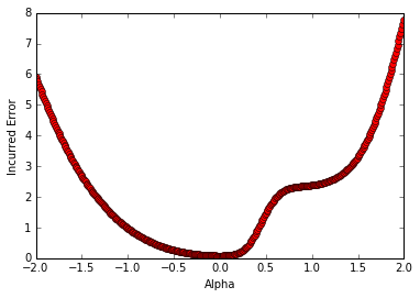
The cost function of a three-layer feed-forward network as we linearly interpolate on the line connecting a randomly initialized parameter vector and an SGD solution

Flat Regions in the Error Surface

More generally, given an arbitrary function, a point at which the gradient is the zero vector is called a critical point.

For a one-dimensional cost function, a critical point can take one of three forms, as shown in Figure 4-4.

4-4

Figure 4-4. Analyzing a critical point along a single dimension

This means given a random critical point in a random one-dimensional function, it has one-third probability of being a local minimum. This means that if we have a total of k critical points, we can expect to have a total of $\frac{k}{3}$ local minima.

We can also extend this to higher dimensional functions. Consider a cost function operating in a d-dimensional space.

4-5

Figure 4-5. A saddle point over a two-dimensional error surface

In general, in a d-dimensional parameter space, we can slice through a critical point on d different axes. A critical point can only be a local minimum if it appears as a local minimum in every single one of the d one-dimensional subspaces. Using the fact that a critical point can come in one of three different flavors(local minima,local maxima and saddle points) in a one-dimensional subspace, we realize that the probability that a random critical point is in a random function is $\frac{1}{3^d}$. This means that a random function function with k critical points has an expected number of $\frac{k}{3^d}$ local minima. In other words, as the dimensionality of our parameter space increases, local minima become exponentially more rare.

It seems like these flat segments of the error surface are pesky but ultimately don’t prevent stochastic gradient descent from converging to a good answer. However, it does pose serious problems for methods that attempt to directly solve for a point where the gradient is zero.

When the Gradient Points in the Wrong Direction

As an example, we consider an error surface defined over a two-dimensional parameter space, as shown in Figure 4-6.

4-6

Figure 4-6. Local information encoded by the gradient usually does not corroborate the global structure of the error surface

Specifically, we realize that only when the contours are perfectly circular does the gradient always point in the direction of the local minimum. However, if the contours are extremely elliptical (as is usually the case for the error surfaces of deep networks), the gradient can be as inaccurate as 90 degrees away from the correct direction!

The general problem with taking a significant step in this direction, however, is that the gradient could be changing under our feet as we move! We demonstrate this simple fact in Figure 4-7. Going back to the two-dimensional example, if our contours are perfectly circular and we take a big step in the direction of the steepest descent, the gradient doesn’t change direction as we move. However, this is not the case for highly elliptical contours.

4-7

Figure 4-7. We show how the direction of the gradient changes as we move along the direction of steepest descent (as determined from a starting point). The gradient vectors are normalized to identical length to emphasize the change in direction of the gradient vector.

More generally, we can quantify how the gradient changes under our feet as we move in a certain direction by computing second derivatives. Specifically, we want to measure $\frac{\partial(\partial E / \partial w_j)}{\partial w_j}$, which tells us how the gradient component for $w_j$ changes as we change the value of $w_i$. We can compile this information into a special matrix known as the Hessian matrix (H). And when describing an error surface where the gradient changes underneath our feet as we move in the direction of steepest descent, this matrix is said to be ill-conditioned.

We can now use a second-order approximation via Taylor series:

$E(x) \approx E(x^{(i)}) + (x-x^{(i)})^T g + \frac{1}{2} (x-x^{(i)})^T H (x-x^{(i)})$

If we go further to state that we will be moving $\epsilon$ units in the direction of the gradient, we can further simplify our expression:

$E(x^{(i)} - \epsilon g) \approx E(x^{(i)}) - \epsilon g^T g + \frac{1}{2}\epsilon^2 g^THg$

This expression consists of three terms:

the value of the error function at the original parameter vector,
the improvement in error afforded by the magnitude of the gradient,
a correction term that incorporates the curvature of the surface as represented by the Hessian matrix.

Momentum-Based Optimization

Fundamentally, the problem of an ill-conditioned Hessian matrix manifests itself in the form of gradients that fluctuate wildly. As a result, one popular mechanism for dealing with ill-conditioning bypasses the computation of the Hessian, and instead, focuses on how to cancel out these fluctuations over the duration of training.

Our goal, then, is to somehow generate an analog for velocity in our optimization algorithm. We can do this by keeping track of an exponentially weighted decay of past gradients. The premise is simple: every update is computed by combining the update in the last iteration with the current gradient. Concretely, we compute the change in the parameter vector as follows:

$v_i = mv_{i-1} - \epsilon g_i$

$\theta_i = \theta_{i-1} + v_i$

In other words, we use the momentum hyperparameter m to determine what fraction of the previous velocity to retain in the new update, and add this “memory” of past gradients to our current gradient. This approach is commonly referred to as momentum.

To better visualize how momentum works, we’ll explore a toy example. Specifically, we’ll investigate how momentum affects updates during a random walk. A random walk is a succession of randomly chosen steps. In our example, we’ll imagine a particle on a line that, at every time interval, randomly picks a step size between -10 and 10 and takes a moves in that direction. This is simply expressed as:

step_range = 10
step_choices = range(-1 * step_range, step_range + 1)
rand_walk = [random.choice(step_choices) for x in xrange(100)]

We’ll then simulate what happens when we use a slight modification of momentum (i.e., the standard exponentially weighted moving average algorithm) to smooth our choice of step at every time interval. Again, we can concisely express this as:

momentum_rand_walk = [random.choice(step_choices)]
for i in xrange(len(rand_walk) - 1):
    prev = momentum_rand_walk[-1]
    rand_choice = random.choice(step_choices)
    new_step = momentum * prev + (1 - momentum) * rand_choice
    momentum_rand_walk.append()

4-8

Figure 4-8. Momentum smooths volatility in the step sizes during a random walk using an exponentially weighted moving average

The resulting speedup is staggering. We display how the cost function changes over time by comparing the TensorBoard visualizations in Figure 4-9. The figure demonstrates that to achieve a cost of 0.1 without momentum (right) requires nearly 18,000 steps (minibatches), whereas with momentum (left), we require just over 2,000.

4-9

Figure 4-9. Comparing training a feed-forward network with (right) and without (left) momentum demonstrates a massive decrease in training time

A Brief View of Second-Order Methods

Several second-order methods, however, have been researched over the past several years that attempt to approximate the Hessian directly.

Conjugate Gradient Descent

In steepest descent, we compute the direction of the gradient and then line search to find the minimum along that direction. We jump to the minimum and then recompute the gradient to determine the direction of the next line search. It turns out that this method ends up zigzagging a significant amount, as shown in Figure 4-9, because each time we move in the direction of steepest descent, we undo a little bit of progress in another direction. A remedy to this problem is moving in a conjugate direction relative to the previous choice instead of the direction of steepest descent. The conjugate direction is chosen by using an indirect approximation of the Hessian to linearly combine the gradient and our previous direction. With a slight modification, this method generalizes to the nonconvex error surfaces we find in deep networks.

4-10

Figure 4-10. The method of steepest descent often zigzags; conjugate descent attempts to remedy this issue

Broyden–Fletcher–Goldfarb–Shanno (BFGS)

BFGS algorithm attempts to compute the inverse of the Hessian matrix iteratively and use the inverse Hessian to more effectively optimize the parameter vector. A more memory-efficient version known as L-BFGS.

Learning Rate Adaptation

AdaGrad—Accumulating Historical Gradients

This learning rate is inversely scaled with respect to the square root of the sum of the squares (root mean square) of all the parameter’s historical gradients.

Flat regions may force AdaGrad to decrease the learning rate before it reaches a minimum.

$r_i=r_{i-1} + g_i \odot g_i$

$r_0=0$
$\odot$ is element-wise tensor multiplication
$g_i \odot g_i$ the square of all the gradient parameters

$\theta_i = \theta_{i-1} - \frac{\epsilon}{\sigma \oplus \sqrt{r_i}} \odot g$

$\epsilon$ global learning rate, is divided by the square root of the gradient accumulation vector
$\sigma(\approx 10^{-7})$ ,a tiny number in order to prevent division by zero

In TensorFlow, a built-in optimizer allows for easily utilizing AdaGrad as a learning algorithm:

tf.train.AdagradOptimizer(learning_rate, 
                          initial_accumulator_value=0.1, 
                          use_locking=False, 
                          name='Adagrad')

the $\epsilon$ and initial gradient accumulation vector are rolled together into the initial_accumulator_value argument

RMSProp—Exponentially Weighted Moving Average of Gradients

$r_i=\rho r_{i-1} + (1 - \rho) g_i \odot g_i$

$\rho$ the decay factor determines how long we keep old gradients

tf.train.RMSPropOptimizer(learning_rate, decay=0.9, 
                          momentum=0.0, epsilon=1e-10, 
                          use_locking=False, name='RMSProp')

Unlike in Adagrad, we pass in $\delta$ separately as the epsilon argument to the constructor.

Adam—Combining Momentum and RMSProp

$\tilde{m_i} = \frac{m_i}{1-\beta_1^i}$

$v_i=\frac{v_i}{1-\beta_2^i}$

$\theta_i=\theta_{i-1} - \frac{\epsilon}{\sigma \oplus \sqrt{v_i}\tilde{m_i}}$

tf.train.AdamOptimizer(learning_rate=0.001, beta1=0.9, 
                       beta2=0.999, epsilon=1e-08, 
                       use_locking=False, name='Adam')

Optimization Algorithms Experiment

!python optimzer_mlp.py sgd

Extracting data/train-images-idx3-ubyte.gz
Extracting data/train-labels-idx1-ubyte.gz
Extracting data/t10k-images-idx3-ubyte.gz
Extracting data/t10k-labels-idx1-ubyte.gz
sgd
2017-08-15 08:28:09.183430: W tensorflow/core/platform/cpu_feature_guard.cc:45] The TensorFlow library wasn't compiled to use SSE4.1 instructions, but these are available on your machine and could speed up CPU computations.
2017-08-15 08:28:09.183453: W tensorflow/core/platform/cpu_feature_guard.cc:45] The TensorFlow library wasn't compiled to use SSE4.2 instructions, but these are available on your machine and could speed up CPU computations.
2017-08-15 08:28:09.183459: W tensorflow/core/platform/cpu_feature_guard.cc:45] The TensorFlow library wasn't compiled to use AVX instructions, but these are available on your machine and could speed up CPU computations.
2017-08-15 08:28:09.183464: W tensorflow/core/platform/cpu_feature_guard.cc:45] The TensorFlow library wasn't compiled to use AVX2 instructions, but these are available on your machine and could speed up CPU computations.
2017-08-15 08:28:09.183469: W tensorflow/core/platform/cpu_feature_guard.cc:45] The TensorFlow library wasn't compiled to use FMA instructions, but these are available on your machine and could speed up CPU computations.
Epoch: 0001 cost = 1.023527871
Validation Error: 0.119799971581
Epoch: 0101 cost = 0.018873566
Validation Error: 0.019200026989
Epoch: 0201 cost = 0.005179930
Validation Error: 0.0184000134468
Epoch: 0301 cost = 0.002607897
Validation Error: 0.0171999931335
Epoch: 0401 cost = 0.001667035
Validation Error: 0.0166000127792
Optimization Finished!
Test Accuracy: 0.9807

!python optimzer_mlp.py momentum

Extracting data/train-images-idx3-ubyte.gz
Extracting data/train-labels-idx1-ubyte.gz
Extracting data/t10k-images-idx3-ubyte.gz
Extracting data/t10k-labels-idx1-ubyte.gz
momentum
2017-08-15 09:07:09.048477: W tensorflow/core/platform/cpu_feature_guard.cc:45] The TensorFlow library wasn't compiled to use SSE4.1 instructions, but these are available on your machine and could speed up CPU computations.
2017-08-15 09:07:09.048500: W tensorflow/core/platform/cpu_feature_guard.cc:45] The TensorFlow library wasn't compiled to use SSE4.2 instructions, but these are available on your machine and could speed up CPU computations.
2017-08-15 09:07:09.048506: W tensorflow/core/platform/cpu_feature_guard.cc:45] The TensorFlow library wasn't compiled to use AVX instructions, but these are available on your machine and could speed up CPU computations.
2017-08-15 09:07:09.048511: W tensorflow/core/platform/cpu_feature_guard.cc:45] The TensorFlow library wasn't compiled to use AVX2 instructions, but these are available on your machine and could speed up CPU computations.
2017-08-15 09:07:09.048515: W tensorflow/core/platform/cpu_feature_guard.cc:45] The TensorFlow library wasn't compiled to use FMA instructions, but these are available on your machine and could speed up CPU computations.
Epoch: 0001 cost = 0.919267848
Validation Error: 0.270600020885
Epoch: 0101 cost = 0.260265864
Validation Error: 0.128000020981
Epoch: 0201 cost = 0.260049450
Validation Error: 0.127799987793
Epoch: 0301 cost = 0.260005093
Validation Error: 0.128199994564
Epoch: 0401 cost = 0.259985650
Validation Error: 0.127799987793
Optimization Finished!
Test Accuracy: 0.8683

Chapter 5. Convolutional Neural Networks

Vanilla Deep Neural Networks Don’t Scale

In MNIST, our images were only 28 x 28 pixels and were black and white. As a result, a neuron in a fully connected hidden layer would have 784 incoming weights. This seems pretty tractable for the MNIST task, and our vanilla neural net performed quite well. This technique, however, does not scale well as our images grow larger. For example, for a full-color 200 x 200 pixel image, our input layer would have 200 x 200 x 3 =120,000 weights.

5-3

Figure 5-3. The density of connections between layers increases intractably as the size of the image increases

As we’ll see, the neurons in a convolutional layer are only connected to a small, local region of the preceding layer. A convolutional layer’s function can be expressed simply: it processes a three-dimensional volume of information to produce a new three-dimensional volume of information.

5-4

Figure 5-4. Convolutional layers arrange neurons in three dimensions, so layers have width, height, and depth

Filters and Feature Maps

A filter is essentially a feature detector.

5-5

Figure 5-5. We’ll analyze this simple black-and-white image as a toy example

Let’s say that we want to detect vertical and horizontal lines in the image. For example, to detect vertical lines, we would use the feature detector on the top, slide it across the entirety of the image, and at every step check if we have a match. This result is our feature map, and it indicates where we’ve found the feature we’re looking for in the original image. We can do the same for the horizontal line detector (bottom), resulting in the feature map in the bottom-right corner.

5-6

Figure 5-6. Applying filters that detect vertical and horizontal lines on our toy example

This operation is called a convolution. We take a filter and we multiply it over the entire area of an input image.

Filters represent combinations of connections (one such combination is highlighted in Figure 5-7) that get replicated across the entirety of the input.

The output layer is the feature map generated by this filter. A neuron in the feature map is activated if the filter contributing to its activity detected an appropriate feature at the corresponding position in the previous layer.

5-7

Figure 5-7. Representing filters and feature maps as neurons in a convolutional layer

Express the feature map as follows:

$m_{ij}^k=f((W \cdot x)_{ij} + b^k)$

the $k^{th}$ feature map in layer m as $m^k$
the corresponding filter by the values of its weights upper W
assuming the neurons in the feature map have bias $b^k$ (note that the bias is kept identical for all of the neurons in a feature map)

And we have accumulated three feature maps, one for eyes, one for noses, and one for mouths. We know that a particular location contains a face if the corresponding locations in the primitive feature maps contain the appropriate features (two eyes, a nose, and a mouth). In other words, to make decisions about the existence of a face, we must combine evidence over multiple feature maps.

As a result, feature maps must be able to operate over volumes, not just areas. This is shown below in Figure 5-8. Each cell in the input volume is a neuron. A local portion is multiplied with a filter (corresponding to weights in the convolutional layer) to produce a neuron in a filter map in the following volumetric layer of neurons.

5-8

Figure 5-8. Representing a full-color RGB image as a volume and applying a volumetric convolutional filter

The depth of the output volume of a convolutional layer is equivalent to the number of filters in that layer, because each filter produces its own slice. We visualize these relationships in Figure 5-9.

5-9

Figure 5-9. A three-dimensional visualization of a convolutional layer, where each filter corresponds to a slice in the resulting output volume

Full Description of the Convolutional Layer

This input volume has the following characteristics:

Its width $w_{in}$
Its height $h_{in}$
Its depth $d_{in}$
Its zero padding p

This volume is processed by a total of k filters, which represent the weights and connections in the convolutional network. These filters have a number of hyperparameters, which are described as follows:

Their spatial extent e, which is equal to the filter’s height and width.
Their stride s, or the distance between consecutive applications of the filter on the input volume. If we use a stride of 1, we get the full convolution described in the previous section. We illustrate this in Figure 5-10.
The bias b (a parameter learned like the values in the filter) which is added to each component of the convolution.

5-10

Figure 5-10. An illustration of a filter’s stride hyperparameter

This results in an output volume with the following characteristics:

Its function f, which is applied to the incoming logit of each neuron in the output volume to determine its final value
Its width $w_{out}=\lceil \frac{w_{in}-e+2p}{s} \rceil + 1$
Its height $h_{out}=\lceil \frac{h_{in}-e+2p}{s} \rceil + 1$
Its depth $d_{out}=k$

5-11

Figure 5-11. This is a convolutional layer with an input volume that has width 5, height 5, depth 3, and zero padding 1. There are 2 filters, with spatial extent 3 and applied with a stride of 2. It results in an output volume with width 3, height 3, and depth 2. We apply the first convolutional filter to the upper-leftmost 3 x 3 piece of the input volume to generate the upper-leftmost entry of the first depth slice.

5-12

Figure 5-12. Using the same setup as Figure 5-11, we generate the next value in the first depth slice of the output volume.

TensorFlow provides us with a convenient operation to easily perform a convolution on a minibatch of input volumes (note that we must apply our choice of function ourselves and it is not performed by the operation itself):

tf.nn.conv2d(input, filter, strides, padding, use_cudnn_on_gpu=True, name=None)

input:a four-dimensional tensor of size $N \times h_{in} \times w_{in} \times d_{in}$, where is the number of examples in our minibatch.
filter:also a four-dimensional tensor representing all of the filters applied in the convolution. It is of size $e \times e \times d_{in} \times k$.
The resulting tensor emitted by this operation has the same structure as input
Setting the padding argument to “SAME” also selects the zero padding so that height and width are preserved by the convolutional layer.

Max Pooling

The essential idea behind max pooling is to break up each feature map into equally sized tiles.Then we create a condensed feature map. Specifically, we create a cell for each tile, compute the maximum value in the tile, and propagate this maximum value into the corresponding cell of the condensed feature map. This process is illustrated in Figure 5-13.

5-13

Figure 5-13. An illustration of how max pooling significantly reduces parameters as we move up the network

We can describe a pooling layer with two parameters:

Its spatial extent e
Its stride s

It’s important to note that only two major variations of the pooling layer are used. The first is the nonoverlapping pooling layer with e = 2, s = 2. The second is the overlapping pooling layer with e = 3， s = 2. The resulting dimensions of each feature map are as follows:

Its width $w_{out}=\lceil \frac{w_{in}-e}{s} \rceil + 1$
Its height $h_{out}=\lceil \frac{h_{in}-e}{s} \rceil + 1$

Full Architectural Description of Convolution Networks

5-14

Figure 5-14. Various convolutional network architectures of various complexities. The architecture of VGGNet, a deep convolutional network built for ImageNet, is shown in the rightmost network.

Closing the Loop on MNIST with Convolutional Networks

We’ll build a convolutional network with a pretty standard architecture (modeled after the second network in Figure 5-14): two pooling and two convolutional interleaved, followed by a fully connected layer (with dropout, p=0.5) and a terminal softmax.

def conv2d(input, weight_shape, bias_shape):
    incoming = weight_shape[0] * weight_shape[1] * weight_shape[2]
    weight_init = tf.random_normal_initializer(stddev=(2.0/incoming)**0.5)
    W = tf.get_variable("W", weight_shape, initializer=weight_init)
    bias_init = tf.constant_initializer(value=0)
    b = tf.get_variable("b", bias_shape, initializer=bias_init)
    return tf.nn.relu(tf.nn.bias_add(tf.nn.conv2d(input, W, strides=[1, 1, 1, 1], padding='SAME'), b))

def max_pool(input, k=2):
    return tf.nn.max_pool(input, ksize=[1, k, k, 1], strides=[1, k, k, 1], padding='SAME')

def layer(input, weight_shape, bias_shape):
    weight_init = tf.random_normal_initializer(stddev=(2.0/weight_shape[0])**0.5)
    bias_init = tf.constant_initializer(value=0)
    W = tf.get_variable("W", weight_shape, initializer=weight_init)
    b = tf.get_variable("b", bias_shape, initializer=bias_init)
    return tf.nn.relu(tf.matmul(input, W) + b)

def inference(x, keep_prob):
    x = tf.reshape(x, shape=[-1, 28, 28, 1])
    with tf.variable_scope("conv_1"):
        conv_1 = conv2d(x, [5, 5, 1, 32], [32])
        pool_1 = max_pool(conv_1)

    with tf.variable_scope("conv_2"):
        conv_2 = conv2d(pool_1, [5, 5, 32, 64], [64])
        pool_2 = max_pool(conv_2)

    with tf.variable_scope("fc"):
        pool_2_flat = tf.reshape(pool_2, [-1, 7 * 7 * 64])
        fc_1 = layer(pool_2_flat, [7*7*64, 1024], [1024])
        
        # apply dropout
        fc_1_drop = tf.nn.dropout(fc_1, keep_prob)

    with tf.variable_scope("output"):
        output = layer(fc_1_drop, [1024, 10], [10])
    return output

def loss(output, y):
    xentropy = tf.nn.softmax_cross_entropy_with_logits(logits=output, labels=y)    
    loss = tf.reduce_mean(xentropy)
    return loss

def training(cost, global_step):
    tf.summary.scalar("cost", cost)
    optimizer = tf.train.AdamOptimizer(learning_rate)
    train_op = optimizer.minimize(cost, global_step=global_step)
    return train_op

def evaluate(output, y):
    correct_prediction = tf.equal(tf.argmax(output, 1), tf.argmax(y, 1))
    accuracy = tf.reduce_mean(tf.cast(correct_prediction, tf.float32))
    tf.summary.scalar("validation error", (1.0 - accuracy))
    return accuracy

Input Layer
- take the flattened versions of the input pixel values and reshape them into a tensor of the $N \times 28 \times 28 \times 1$, where
  - N is the number of examples in a minibatch,
  - 28 is the width and height of each image, and
  - 1 is the depth (because the images are black and white; if the images were in RGB color, the depth would instead be 3 to represent each color map).
Conv Layer
- build a convolutional layer with 32 filters that have spatial extent 5.
- results in taking an input volume of depth 1 and emitting a output tensor of depth 32.
Max Pooling
- then passed through a max pooling layer which compresses the information.
Conv Layer2
- build a second convolutional layer with 64 filters, again with spatial extent 5, taking an input tensor of depth 32 and emitting an output tensor of depth 64.
Max Pooling
- passed through a max pooling layer to compress information.

import input_data
mnist = input_data.read_data_sets("data/", one_hot=True)

import tensorflow as tf

# Architecture
n_hidden_1 = 256
n_hidden_2 = 256

# Parameters
learning_rate = 0.0001
training_epochs = 1000
batch_size = 100
display_step = 10

with tf.device("/gpu:0"):
    with tf.Graph().as_default():
        with tf.variable_scope("mnist_conv_model"):
            x = tf.placeholder("float", [None, 784]) # mnist data image of shape 28*28=784
            y = tf.placeholder("float", [None, 10]) # 0-9 digits recognition => 10 classes
            keep_prob = tf.placeholder(tf.float32) # dropout probability

            output = inference(x, keep_prob)
            cost = loss(output, y)
            global_step = tf.Variable(0, name='global_step', trainable=False)
            train_op = training(cost, global_step)
            eval_op = evaluate(output, y)
            summary_op = tf.summary.merge_all()
            saver = tf.train.Saver()

            sess = tf.Session()
            summary_writer = tf.summary.FileWriter("conv_mnist_logs/", graph=sess.graph)

            init_op = tf.global_variables_initializer()
            sess.run(init_op)

            # Training cycle
            for epoch in range(training_epochs):
                avg_cost = 0.
                total_batch = int(mnist.train.num_examples/batch_size)
                # Loop over all batches
                for i in range(total_batch):
                    minibatch_x, minibatch_y = mnist.train.next_batch(batch_size)
                    # Fit training using batch data
                    sess.run(train_op, feed_dict={x: minibatch_x, y: minibatch_y, keep_prob: 0.5})
                    # Compute average loss
                    avg_cost += sess.run(cost, feed_dict={x: minibatch_x, y: minibatch_y, keep_prob: 0.5})/total_batch
                # Display logs per epoch step
                if epoch % display_step == 0:
                    print "Epoch:", '%04d' % (epoch+1), "cost =", "{:.9f}".format(avg_cost)
                    accuracy = sess.run(eval_op, feed_dict={x: mnist.validation.images, y: mnist.validation.labels, keep_prob: 1})
                    print "Validation Error:", (1 - accuracy)

                    summary_str = sess.run(summary_op, feed_dict={x: minibatch_x, y: minibatch_y, keep_prob: 0.5})
                    summary_writer.add_summary(summary_str, sess.run(global_step))
                    saver.save(sess, "conv_mnist_logs/model-checkpoint", global_step=global_step)

            print "Optimization Finished!"
            accuracy = sess.run(eval_op, feed_dict={x: mnist.test.images, y: mnist.test.labels, keep_prob: 1})
            print "Test Accuracy:", accuracy

Building a Convolutional Network for CIFAR-10

The CIFAR-10 challenge consists of 32 x 32 color images that belong to one of 10 possible classes.

Normalization of image inputs helps out the training process by making it more robust to variations. Batch normalization takes this a step further by normalizing inputs to every layer in our neural network. Specifically, we modify the architecture of our network to include operations that:

Grab the vector of logits incoming to a layer before they pass through the nonlinearity
Normalize each component of the vector of logits across all examples of the minibatch by subtracting the mean and dividing by the standard deviation (we keep track of the moments using an exponentially weighted moving average)
Given normalized inputs x̂, use an affine transform to restore representational power with two vectors of (trainable) parameters: γx̂ + β

Expressed in TensorFlow, batch normalization can be expressed as follows for a convolutional layer:

def conv_batch_norm(x, n_out, phase_train):
    beta_init = tf.constant_initializer(value=0.0, dtype=tf.float32)
    gamma_init = tf.constant_initializer(value=1.0, dtype=tf.float32)

    beta = tf.get_variable("beta", [n_out], initializer=beta_init)
    gamma = tf.get_variable("gamma", [n_out], initializer=gamma_init)

    batch_mean, batch_var = tf.nn.moments(x, [0,1,2], name='moments')
    ema = tf.train.ExponentialMovingAverage(decay=0.9)
    ema_apply_op = ema.apply([batch_mean, batch_var])
    ema_mean, ema_var = ema.average(batch_mean), ema.average(batch_var)

    def mean_var_with_update():
        with tf.control_dependencies([ema_apply_op]):
            return tf.identity(batch_mean), tf.identity(batch_var)

    mean, var = control_flow_ops.cond(phase_train,
        mean_var_with_update,
        lambda: (ema_mean, ema_var))

    normed = tf.nn.batch_norm_with_global_normalization(x, mean, var, beta, gamma, 1e-3, True)
    return normed

Non-Batch:convnet_cifar.py

import cifar10_input
cifar10_input.maybe_download_and_extract()

import tensorflow as tf
import numpy as np
import time, os

# Architecture
n_hidden_1 = 256
n_hidden_2 = 256

# Parameters
learning_rate = 0.001
training_epochs = 1000
batch_size = 128
display_step = 1

def inputs(eval_data=True):
    data_dir = os.path.join('data/cifar10_data', 'cifar-10-batches-bin')
    return cifar10_input.inputs(eval_data=eval_data, data_dir=data_dir, batch_size=batch_size)

def distorted_inputs():
    data_dir = os.path.join('data/cifar10_data', 'cifar-10-batches-bin')
    return cifar10_input.distorted_inputs(data_dir=data_dir, batch_size=batch_size)

def filter_summary(V, weight_shape):
    ix = weight_shape[0]
    iy = weight_shape[1]
    cx, cy = 8, 8
    V_T = tf.transpose(V, (3, 0, 1, 2))
    tf.image_summary("filters", V_T, max_images=64) 

def conv2d(input, weight_shape, bias_shape, visualize=False):
    incoming = weight_shape[0] * weight_shape[1] * weight_shape[2]
    weight_init = tf.random_normal_initializer(stddev=(2.0/incoming)**0.5)
    W = tf.get_variable("W", weight_shape, initializer=weight_init)
    if visualize:
        filter_summary(W, weight_shape)
    bias_init = tf.constant_initializer(value=0)
    b = tf.get_variable("b", bias_shape, initializer=bias_init)
    return tf.nn.relu(tf.nn.bias_add(tf.nn.conv2d(input, W, strides=[1, 1, 1, 1], padding='SAME'), b))

def max_pool(input, k=2):
    return tf.nn.max_pool(input, ksize=[1, k, k, 1], strides=[1, k, k, 1], padding='SAME')

def layer(input, weight_shape, bias_shape):
    weight_init = tf.random_normal_initializer(stddev=(2.0/weight_shape[0])**0.5)
    bias_init = tf.constant_initializer(value=0)
    W = tf.get_variable("W", weight_shape,
                        initializer=weight_init)
    b = tf.get_variable("b", bias_shape,
                        initializer=bias_init)
    return tf.nn.relu(tf.matmul(input, W) + b)

def inference(x, keep_prob):
    with tf.variable_scope("conv_1"):
        conv_1 = conv2d(x, [5, 5, 3, 64], [64], visualize=True)
        pool_1 = max_pool(conv_1)

    with tf.variable_scope("conv_2"):
        conv_2 = conv2d(pool_1, [5, 5, 64, 64], [64])
        pool_2 = max_pool(conv_2)

    with tf.variable_scope("fc_1"):
        dim = 1
        for d in pool_2.get_shape()[1:].as_list():
            dim *= d

        pool_2_flat = tf.reshape(pool_2, [-1, dim])
        fc_1 = layer(pool_2_flat, [dim, 384], [384])
        
        # apply dropout
        fc_1_drop = tf.nn.dropout(fc_1, keep_prob)

    with tf.variable_scope("fc_2"):
        fc_2 = layer(fc_1_drop, [384, 192], [192])
        # apply dropout
        fc_2_drop = tf.nn.dropout(fc_2, keep_prob)

    with tf.variable_scope("output"):
        output = layer(fc_2_drop, [192, 10], [10])
    return output


def loss(output, y):
    xentropy = tf.nn.sparse_softmax_cross_entropy_with_logits(output, tf.cast(y, tf.int64))    
    loss = tf.reduce_mean(xentropy)
    return loss

def training(cost, global_step):
    tf.scalar_summary("cost", cost)
    optimizer = tf.train.AdamOptimizer(learning_rate)
    train_op = optimizer.minimize(cost, global_step=global_step)
    return train_op

def evaluate(output, y):
    correct_prediction = tf.equal(tf.cast(tf.argmax(output, 1), dtype=tf.int32), y)
    accuracy = tf.reduce_mean(tf.cast(correct_prediction, tf.float32))
    tf.scalar_summary("validation error", (1.0 - accuracy))
    return accuracy

if __name__ == '__main__':
    with tf.device("/gpu:0"):
        with tf.Graph().as_default():
            with tf.variable_scope("cifar_conv_model"):

                x = tf.placeholder("float", [None, 24, 24, 3])
                y = tf.placeholder("int32", [None])
                keep_prob = tf.placeholder(tf.float32) # dropout probability

                distorted_images, distorted_labels = distorted_inputs()
                val_images, val_labels = inputs()

                output = inference(x, keep_prob)

                cost = loss(output, y)

                global_step = tf.Variable(0, name='global_step', trainable=False)

                train_op = training(cost, global_step)

                eval_op = evaluate(output, y)

                summary_op = tf.summary.merge_all()

                saver = tf.train.Saver()

                sess = tf.Session()

                summary_writer = tf.summary.FileWriter("conv_cifar_logs/", graph=sess.graph)

                init_op = tf.global_variables_initializer()

                sess.run(init_op)

                tf.train.start_queue_runners(sess=sess)

                # Training cycle
                for epoch in range(training_epochs):

                    avg_cost = 0.
                    total_batch = int(cifar10_input.NUM_EXAMPLES_PER_EPOCH_FOR_TRAIN/batch_size)
                    # Loop over all batches
                    for i in range(total_batch):
                        # Fit training using batch data

                        train_x, train_y = sess.run([distorted_images, distorted_labels])

                        _, new_cost = sess.run([train_op, cost], feed_dict={x: train_x, y: train_y, keep_prob: 0.5})
                        # Compute average loss
                        avg_cost += new_cost/total_batch
                        # print "Epoch %d, minibatch %d of %d. Cost = %0.4f." %(epoch, i, total_batch, new_cost)
                    
                    # Display logs per epoch step
                    if epoch % display_step == 0:
                        print "Epoch:", '%04d' % (epoch+1), "cost =", "{:.9f}".format(avg_cost)

                        val_x, val_y = sess.run([val_images, val_labels])

                        accuracy = sess.run(eval_op, feed_dict={x: val_x, y: val_y, keep_prob: 1})

                        print "Validation Error:", (1 - accuracy)

                        summary_str = sess.run(summary_op, feed_dict={x: train_x, y: train_y, keep_prob: 1})
                        summary_writer.add_summary(summary_str, sess.run(global_step))

                        saver.save(sess, "conv_cifar_logs/model-checkpoint", global_step=global_step)

                print "Optimization Finished!"
                val_x, val_y = sess.run([val_images, val_labels])
                accuracy = sess.run(eval_op, feed_dict={x: val_x, y: val_y, keep_prob: 1})
                print "Test Accuracy:", accuracy

Batch:

def conv_batch_norm(x, n_out, phase_train):
    beta_init = tf.constant_initializer(value=0.0, dtype=tf.float32)
    gamma_init = tf.constant_initializer(value=1.0, dtype=tf.float32)

    beta = tf.get_variable("beta", [n_out], initializer=beta_init)
    gamma = tf.get_variable("gamma", [n_out], initializer=gamma_init)

    batch_mean, batch_var = tf.nn.moments(x, [0,1,2], name='moments')
    ema = tf.train.ExponentialMovingAverage(decay=0.9)
    ema_apply_op = ema.apply([batch_mean, batch_var])
    ema_mean, ema_var = ema.average(batch_mean), ema.average(batch_var)
    def mean_var_with_update():
        with tf.control_dependencies([ema_apply_op]):
            return tf.identity(batch_mean), tf.identity(batch_var)
    mean, var = control_flow_ops.cond(phase_train,
        mean_var_with_update,
        lambda: (ema_mean, ema_var))

    normed = tf.nn.batch_norm_with_global_normalization(x, mean, var,
        beta, gamma, 1e-3, True)
    return normed

def layer_batch_norm(x, n_out, phase_train):
    beta_init = tf.constant_initializer(value=0.0, dtype=tf.float32)
    gamma_init = tf.constant_initializer(value=1.0, dtype=tf.float32)

    beta = tf.get_variable("beta", [n_out], initializer=beta_init)
    gamma = tf.get_variable("gamma", [n_out], initializer=gamma_init)

    batch_mean, batch_var = tf.nn.moments(x, [0], name='moments')
    ema = tf.train.ExponentialMovingAverage(decay=0.9)
    ema_apply_op = ema.apply([batch_mean, batch_var])
    ema_mean, ema_var = ema.average(batch_mean), ema.average(batch_var)
    def mean_var_with_update():
        with tf.control_dependencies([ema_apply_op]):
            return tf.identity(batch_mean), tf.identity(batch_var)
    mean, var = control_flow_ops.cond(phase_train,
        mean_var_with_update,
        lambda: (ema_mean, ema_var))

    reshaped_x = tf.reshape(x, [-1, 1, 1, n_out])
    normed = tf.nn.batch_norm_with_global_normalization(reshaped_x, mean, var,
        beta, gamma, 1e-3, True)
    return tf.reshape(normed, [-1, n_out])

def filter_summary(V, weight_shape):
    ix = weight_shape[0]
    iy = weight_shape[1]
    cx, cy = 8, 8
    V_T = tf.transpose(V, (3, 0, 1, 2))
    tf.image_summary("filters", V_T, max_images=64) 

def conv2d(input, weight_shape, bias_shape, phase_train, visualize=False):
    incoming = weight_shape[0] * weight_shape[1] * weight_shape[2]
    weight_init = tf.random_normal_initializer(stddev=(2.0/incoming)**0.5)
    W = tf.get_variable("W", weight_shape, initializer=weight_init)
    if visualize:
        filter_summary(W, weight_shape)
    bias_init = tf.constant_initializer(value=0)
    b = tf.get_variable("b", bias_shape, initializer=bias_init)
    logits = tf.nn.bias_add(tf.nn.conv2d(input, W, strides=[1, 1, 1, 1], padding='SAME'), b)
    return tf.nn.relu(conv_batch_norm(logits, weight_shape[3], phase_train))

def max_pool(input, k=2):
    return tf.nn.max_pool(input, ksize=[1, k, k, 1], strides=[1, k, k, 1], padding='SAME')

def layer(input, weight_shape, bias_shape, phase_train):
    weight_init = tf.random_normal_initializer(stddev=(2.0/weight_shape[0])**0.5)
    bias_init = tf.constant_initializer(value=0)
    W = tf.get_variable("W", weight_shape, initializer=weight_init)
    b = tf.get_variable("b", bias_shape, initializer=bias_init)
    logits = tf.matmul(input, W) + b
    return tf.nn.relu(layer_batch_norm(logits, weight_shape[1], phase_train))

def inference(x, keep_prob, phase_train):
    with tf.variable_scope("conv_1"):
        conv_1 = conv2d(x, [5, 5, 3, 64], [64], phase_train, visualize=True)
        pool_1 = max_pool(conv_1)

    with tf.variable_scope("conv_2"):
        conv_2 = conv2d(pool_1, [5, 5, 64, 64], [64], phase_train)
        pool_2 = max_pool(conv_2)

    with tf.variable_scope("fc_1"):
        dim = 1
        for d in pool_2.get_shape()[1:].as_list():
            dim *= d

        pool_2_flat = tf.reshape(pool_2, [-1, dim])
        fc_1 = layer(pool_2_flat, [dim, 384], [384], phase_train)
        
        # apply dropout
        fc_1_drop = tf.nn.dropout(fc_1, keep_prob)

    with tf.variable_scope("fc_2"):
        fc_2 = layer(fc_1_drop, [384, 192], [192], phase_train)
        # apply dropout
        fc_2_drop = tf.nn.dropout(fc_2, keep_prob)

    with tf.variable_scope("output"):
        output = layer(fc_2_drop, [192, 10], [10], phase_train)

    return output

def loss(output, y):
    xentropy = tf.nn.sparse_softmax_cross_entropy_with_logits(output, tf.cast(y, tf.int64))    
    loss = tf.reduce_mean(xentropy)
    return loss

def training(cost, global_step):
    tf.scalar_summary("cost", cost)
    optimizer = tf.train.AdamOptimizer(learning_rate)
    train_op = optimizer.minimize(cost, global_step=global_step)
    return train_op

def evaluate(output, y):
    correct_prediction = tf.equal(tf.cast(tf.argmax(output, 1), dtype=tf.int32), y)
    accuracy = tf.reduce_mean(tf.cast(correct_prediction, tf.float32))
    tf.scalar_summary("validation error", (1.0 - accuracy))
    return accuracy

we integrate batch normalization into the convolutional and fully connected layers
use two convolutional layers (each followed by a max pooling layer)
two fully connected layers followed by a softmax
dropout is included for reference, but in the batch normalization version, keep_prob=1 during training

import cifar10_input
cifar10_input.maybe_download_and_extract()

import tensorflow as tf
from tensorflow.python import control_flow_ops
import numpy as np
import os

# Architecture
n_hidden_1 = 256
n_hidden_2 = 256

# Parameters
learning_rate = 0.01
training_epochs = 1000
batch_size = 128
display_step = 1

def inputs(eval_data=True):
    data_dir = os.path.join('data/cifar10_data', 'cifar-10-batches-bin')
    return cifar10_input.inputs(eval_data=eval_data, data_dir=data_dir,
                                batch_size=batch_size)

def distorted_inputs():
    data_dir = os.path.join('data/cifar10_data', 'cifar-10-batches-bin')
    return cifar10_input.distorted_inputs(data_dir=data_dir,
                                          batch_size=batch_size)

with tf.device("/gpu:0"):
    with tf.Graph().as_default():
        with tf.variable_scope("cifar_conv_bn_model"):
            x = tf.placeholder("float", [None, 24, 24, 3])
            y = tf.placeholder("int32", [None])
            keep_prob = tf.placeholder(tf.float32) # dropout probability
            phase_train = tf.placeholder(tf.bool) # training or testing

            distorted_images, distorted_labels = distorted_inputs()
            val_images, val_labels = inputs()

            output = inference(x, keep_prob, phase_train)
            cost = loss(output, y)
            global_step = tf.Variable(0, name='global_step', trainable=False)
            train_op = training(cost, global_step)
            eval_op = evaluate(output, y)

            summary_op = tf.summary.merge_all()

            saver = tf.train.Saver()
            sess = tf.Session()

            summary_writer = tf.summary.FileWriter("conv_cifar_bn_logs/", graph=sess.graph)
            init_op = tf.global_variables_initializer()
            sess.run(init_op)
            tf.train.start_queue_runners(sess=sess)

            # Training cycle
            for epoch in range(training_epochs):
                avg_cost = 0.
                total_batch = int(cifar10_input.NUM_EXAMPLES_PER_EPOCH_FOR_TRAIN/batch_size)
                # Loop over all batches
                for i in range(total_batch):
                    # Fit training using batch data

                    train_x, train_y = sess.run([distorted_images, distorted_labels])
                    _, new_cost = sess.run([train_op, cost], feed_dict={x: train_x, y: train_y, keep_prob: 1, phase_train: True})
                    # Compute average loss
                    avg_cost += new_cost/total_batch
                    print "Epoch %d, minibatch %d of %d. Cost = %0.4f." %(epoch, i, total_batch, new_cost)

                # Display logs per epoch step
                if epoch % display_step == 0:
                    print "Epoch:", '%04d' % (epoch+1), "cost =", "{:.9f}".format(avg_cost)
                    val_x, val_y = sess.run([val_images, val_labels])
                    accuracy = sess.run(eval_op, feed_dict={x: val_x, y: val_y, keep_prob: 1, phase_train: False})
                    print "Validation Error:", (1 - accuracy)

                    summary_str = sess.run(summary_op, feed_dict={x: train_x, y: train_y, keep_prob: 1, phase_train: False})
                    summary_writer.add_summary(summary_str, sess.run(global_step))
                    saver.save(sess, "conv_cifar_bn_logs/model-checkpoint", global_step=global_step)

            print "Optimization Finished!"
            val_x, val_y = sess.run([val_images, val_labels])
            accuracy = sess.run(eval_op, feed_dict={x: val_x, y: val_y, keep_prob: 1, phase_train: False})
            print "Test Accuracy:", accuracy

Visualizing Learning in Convolutional Networks

5-17

Figure 5-17. Training a convolutional network without batch normalization (left) versus with batch normalization (right). Batch normalization vastly accelerates the training process.

5-18

Figure 5-18. A subset of the learned filters in the first convolutional layer of our network

We then take this high-dimensional representation for each image and use an algorithm known as t-Distributed Stochastic Neighbor Embedding, or t-SNE, to compress it to a two-dimensional representation that we can visualize.

5-19

Figure 5-19. The t-SNE embedding (center) surrounded by zoomed-in subsegments of the embedding (periphery).

Leveraging Convolutional Filters to Replicate Artistic Styles

The goal of neural style is to be able to take an arbitrary photograph and re-render it as if it were painted in the style of a famous artist.

Let’s take a pre-trained convolutional network. There are three images that we’re dealing with. The first two are the source of content p and the source of style a. The third image is the generated image x. Our goal will be to derive an error function that we can backpropagate that, when minimized, will perfectly combine the content of the desired photograph and the style of the desired artwork.

We start with content first. If a layer in the network has $k_l$ filters, then it produces a total of $k_l$ feature maps. Let’s call the size of each feature map $m_l$, the height times the width of the feature map. This means that the activations in all the feature maps of this layer can be stored in a matrix $F^{(l)}$ of size $k_l \times m_l$. We can also represent all the activations of the photograph in a matrix $P^{(l)}$ and all the activations of the generated image in the matrix $X^{(l)}$. We use the relu4_2 of the original VGGNet:

$E_{content}(p,x)=\sum_{ij}(P_{ij}^{(l)}-X_{ij}^{(l)})^2$

Now we can try tackling style. To do this we construct a matrix known as the Gram matrix, which represents correlations between feature maps in a given layer. The correlations represent the texture and feel that is common among all features, irrespective of which features we’re looking at. Constructing the Gram matrix, which is of size $k_l \times k_l$, for a given image is done as follows:

$G_{ij}^{(l)}=\sum_{c=0}^{m_l} F_{ic}^{(l)}F_{jc}^{(l)}$

We can compute the Gram matrices for both the artwork in matrix $A^{(l)}$ and the generated image in $G^{(l)}$. We can then represent the error function as:

$E_{style}(a,x)=\frac{1}{4k_l^2m_l^2}\sum_{l=1}^L \sum_{ij}\frac{1}{L}(A_{ij}^{(l)}-G_{ij}^{(l)})^2$

TensorFlow code (https://github.com/darksigma/Fundamentals-of-Deep-Learning-Book/tree/master/archive/neural_style)

5-20

Figure 5-20. The result of mixing the Rain Princess with a photograph of the MIT Dome. Image credit: Anish Athalye.

Chapter 6. Embedding and Representation Learning

Learning Lower-Dimensional Representations

6-1

Figure 6-1. Using embeddings to automate feature selection in the face of scarce labeled data

Principal Component Analysis

More specifically, if we have d-dimensional data, we’d like to find a new set of m < d dimensions that conserves as much valuable information from the original dataset.

First we find a unit vector along which the dataset has maximum variance. Because this direction contains the most information, we select this direction as our first axis. Then from the set of vectors orthogonal to this first choice, we pick a new unit vector along which the dataset has maximum variance. This is our second axis. We continue this process until we have found a total of d new vectors that represent new axes. We project our data onto this new set of axes. We then decide a good value for m and toss out all but the first m axes (the principal components, which store the most information). The result is shown in Figure 6-2.

6-2

Figure 6-2. An illustration of PCA for dimensionality reduction to capture the dimension with the most information (as proxied by variance)

While PCA has been used for decades for dimensionality reduction, it spectacularly fails to capture important relationships that are piecewise linear or nonlinear.

6-3

Figure 6-3. A situation in which PCA fails to optimally transform the data for dimensionality reduction

Motivating the Autoencoder Architecture

6-4

Figure 6-4. The autoencoder architecture attempts to construct a high-dimensional input into a low-dimensional embedding and then uses that low-dimensional embedding to reconstruct the input

Implementing an Autoencoder in TensorFlow

“Reducing the dimensionality of data with neural networks”(Hinton and Salakhutdinov in 2006):Their hypothesis was that the nonlinear complexities afforded by a neural model would allow them to capture structure that linear methods, such as PCA, would miss.

6-5

Figure 6-5. The experimental setup for dimensionality reduction of the MNIST dataset employed by Hinton and Salakhutdinov, 2006

%matplotlib inline

def layer_batch_norm(x, n_out, phase_train):
    beta_init = tf.constant_initializer(value=0.0, dtype=tf.float32)
    gamma_init = tf.constant_initializer(value=1.0, dtype=tf.float32)

    beta = tf.get_variable("beta", [n_out], initializer=beta_init)
    gamma = tf.get_variable("gamma", [n_out], initializer=gamma_init)

    batch_mean, batch_var = tf.nn.moments(x, [0], name='moments')
    ema = tf.train.ExponentialMovingAverage(decay=0.9)
    ema_apply_op = ema.apply([batch_mean, batch_var])
    ema_mean, ema_var = ema.average(batch_mean), ema.average(batch_var)
    def mean_var_with_update():
        with tf.control_dependencies([ema_apply_op]):
            return tf.identity(batch_mean), tf.identity(batch_var)
    mean, var = tf.cond(phase_train,
        mean_var_with_update,
        lambda: (ema_mean, ema_var))

    reshaped_x = tf.reshape(x, [-1, 1, 1, n_out])
    normed = tf.nn.batch_norm_with_global_normalization(reshaped_x, mean, var,
        beta, gamma, 1e-3, True)
    return tf.reshape(normed, [-1, n_out])

def layer(input, weight_shape, bias_shape, phase_train):
    weight_init = tf.random_normal_initializer(stddev=(2.0/weight_shape[0])**0.5)
    bias_init = tf.constant_initializer(value=0)
    W = tf.get_variable("W", weight_shape, initializer=weight_init)
    b = tf.get_variable("b", bias_shape, initializer=bias_init)
    logits = tf.matmul(input, W) + b
    return tf.nn.relu(layer_batch_norm(logits, weight_shape[1], phase_train))

def encoder(x, phase_train):
    with tf.variable_scope("encoder"):
        with tf.variable_scope("hidden_1"):
            hidden_1 = layer(x, [784, n_encoder_hidden_1], [n_encoder_hidden_1], phase_train)
         
        with tf.variable_scope("hidden_2"):
            hidden_2 = layer(hidden_1, [n_encoder_hidden_1, n_encoder_hidden_2], [n_encoder_hidden_2], phase_train)
         
        with tf.variable_scope("hidden_3"):
            hidden_3 = layer(hidden_2, [n_encoder_hidden_2, n_encoder_hidden_3], [n_encoder_hidden_3], phase_train)

        with tf.variable_scope("code"):
            code = layer(hidden_3, [n_encoder_hidden_3, n_code], [n_code], phase_train)

    return code

def decoder(code, phase_train):
    with tf.variable_scope("decoder"):
        with tf.variable_scope("hidden_1"):
            hidden_1 = layer(code, [n_code, n_decoder_hidden_1], [n_decoder_hidden_1], phase_train)
         
        with tf.variable_scope("hidden_2"):
            hidden_2 = layer(hidden_1, [n_decoder_hidden_1, n_decoder_hidden_2], [n_decoder_hidden_2], phase_train)
         
        with tf.variable_scope("hidden_3"):
            hidden_3 = layer(hidden_2, [n_decoder_hidden_2, n_decoder_hidden_3], [n_decoder_hidden_3], phase_train)

        with tf.variable_scope("output"):
            output = layer(hidden_3, [n_decoder_hidden_3, 784], [784], phase_train)

    return output

def loss(output, x):
    with tf.variable_scope("training"):
        l2 = tf.sqrt(tf.reduce_sum(tf.square(tf.subtract(output, x)), 1))
        train_loss = tf.reduce_mean(l2)
        train_summary_op = tf.summary.scalar("train_cost", train_loss)
        return train_loss, train_summary_op

def training(cost, global_step):
    optimizer = tf.train.AdamOptimizer(learning_rate=0.001, beta1=0.9, beta2=0.999, epsilon=1e-08, 
        use_locking=False, name='Adam')
    train_op = optimizer.minimize(cost, global_step=global_step)
    return train_op

def image_summary(label, tensor):
    tensor_reshaped = tf.reshape(tensor, [-1, 28, 28, 1])
    return tf.summary.image(label, tensor_reshaped)

def evaluate(output, x):
    with tf.variable_scope("validation"):
        in_im_op = image_summary("input_image", x)
        out_im_op = image_summary("output_image", output)
        l2 = tf.sqrt(tf.reduce_sum(tf.square(tf.subtract(output, x, name="val_diff")), 1))
        val_loss = tf.reduce_mean(l2)
        val_summary_op = tf.summary.scalar("val_cost", val_loss)
        return val_loss, in_im_op, out_im_op, val_summary_op

The output of the decoder network is a 784-dimensional vector that can be reconstructed into a 28 × 28 image.
In order to accelerate training, we’ll reuse the batch normalization strategy we employed in Chapter 5.
Loss
- Given an input vector upper I and a reconstruction upper O
- $\lVert I-O \rVert=\sqrt{\sum_i(I_i-O_i)^2}$, also known as the L2 norm of the difference between the two vectors
Evaluate
- Use a validation dataset and compute the same L2 norm measurement for model evaluation.
- Collect image summaries so that we can compare both the input images and the reconstructions.

import input_data
mnist = input_data.read_data_sets("data/", one_hot=True)

import tensorflow as tf

# Architecture
n_encoder_hidden_1 = 1000
n_encoder_hidden_2 = 500
n_encoder_hidden_3 = 250
n_code = 30
n_decoder_hidden_1 = 250
n_decoder_hidden_2 = 500
n_decoder_hidden_3 = 1000

# Parameters
learning_rate = 0.01
training_epochs = 500
batch_size = 100
display_step = 100

with tf.Graph().as_default():
    with tf.variable_scope("autoencoder_model"):
        x = tf.placeholder("float", [None, 784]) # mnist data image of shape 28*28=784
        phase_train = tf.placeholder(tf.bool)

        code = encoder(x, phase_train)
        output = decoder(code, phase_train)
        cost, train_summary_op = loss(output, x)
        global_step = tf.Variable(0, name='global_step', trainable=False)
        train_op = training(cost, global_step)
        eval_op, in_im_op, out_im_op, val_summary_op = evaluate(output, x)
        summary_op = tf.summary.merge_all()

        saver = tf.train.Saver()
        sess = tf.Session()
        train_writer = tf.summary.FileWriter("mnist_autoencoder_logs/", graph=sess.graph)
        val_writer = tf.summary.FileWriter("mnist_autoencoder_logs/",graph=sess.graph)

        init_op = tf.global_variables_initializer()
        sess.run(init_op)

        # Training cycle
        for epoch in range(training_epochs):
            avg_cost = 0.
            total_batch = int(mnist.train.num_examples/batch_size)
            # Loop over all batches
            for i in range(total_batch):
                minibatch_x, minibatch_y = mnist.train.next_batch(batch_size)
                # Fit training using batch data
                _, new_cost, train_summary = sess.run([train_op, cost, train_summary_op], feed_dict={x: minibatch_x, phase_train: True})
                train_writer.add_summary(train_summary, sess.run(global_step))
                # Compute average loss
                avg_cost += new_cost/total_batch
            # Display logs per epoch step
            if epoch % display_step == 0:
                print "Epoch:", '%04d' % (epoch+1), "cost =", "{:.9f}".format(avg_cost)

                validation_loss, in_im, out_im, val_summary = sess.run([eval_op, in_im_op, out_im_op, val_summary_op], feed_dict={x: mnist.validation.images, phase_train: False})
                val_writer.add_summary(in_im, sess.run(global_step))
                val_writer.add_summary(out_im, sess.run(global_step))
                val_writer.add_summary(val_summary, sess.run(global_step))
                print "Validation Loss:", validation_loss
                saver.save(sess, "mnist_autoencoder_logs/model-checkpoint", global_step=global_step)

        print "Optimization Finished!"
        test_loss = sess.run(eval_op, feed_dict={x: mnist.test.images, phase_train: False})
        print "Test Loss:", loss

Extracting data/train-images-idx3-ubyte.gz
Extracting data/train-labels-idx1-ubyte.gz
Extracting data/t10k-images-idx3-ubyte.gz
Extracting data/t10k-labels-idx1-ubyte.gz
Epoch: 0001 cost = 5.726947857
Validation Loss: 4.45524
Epoch: 0101 cost = 1.875294229
Validation Loss: 1.81979
Epoch: 0201 cost = 1.757120199
Validation Loss: 1.76411
Epoch: 0301 cost = 1.665520479
Validation Loss: 1.77019
Epoch: 0401 cost = 1.611918144
Validation Loss: 1.75243
Optimization Finished!
Test Loss: <function loss at 0x10462baa0>

The reconstructions for three randomly chosen samples from the test set are shown in Figure 6-9.

6-9

Figure 6-9. A side-by-side comparison of the original inputs (from the validation set) and reconstructions after 5, 100, and 200 epochs of training

from sklearn import decomposition
import input_data

mnist = input_data.read_data_sets("data/", one_hot=False)
pca = decomposition.PCA(n_components=2)
pca.fit(mnist.train.images)
pca_codes = pca.transform(mnist.test.images)

Extracting data/train-images-idx3-ubyte.gz
Extracting data/train-labels-idx1-ubyte.gz
Extracting data/t10k-images-idx3-ubyte.gz
Extracting data/t10k-labels-idx1-ubyte.gz

one_hot=False:labels to be provided as integers instead of one-hot vectors.
n_components=2:to generate two-dimensional codes.

We can also reconstruct the original images from the two-dimensional codes and visualize the reconstructions:

from matplotlib import pyplot as plt

pca_recon = pca.inverse_transform(pca_codes[:1])
plt.imshow(pca_recon[0].reshape((28,28)), cmap=plt.cm.gray)
plt.show()

pca

6-10

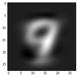
Figure 6-10. Comparing the reconstructions by both PCA and autoencoder side by side

In the resulting visualization in Figure 6-11, it is extremely difficult to make out separable clusters in the two-dimensional PCA codes; the autoencoder has clearly done a spectacular job at clustering codes of different digit classes. This means that a simple machine learning model is going to be able to much more effectively classify data points consisting of autoencoder embeddings as compared to PCA embeddings.

6-11

Figure 6-11. We visualize two-dimensional embeddings produced by PCA (left) and by an autoencoder (right). Notice that the autoencoder does a much better job of clustering codes of different digit classes.

Denoising to Force Robust Representations

6-12

Figure 6-12. In the top row, we have original images from the MNIST dataset. In the bottom row, we’ve randomly blacked out half of the pixels. Despite the corruption, the digits in the bottom row are still identifiable by human perception.

This is a property we might hope to enforce in our embedding algorithm, and it was first explored by Vincent et al. in 2008, when they introduced the denoising autoencoder.

Let’s say we had a two-dimensional dataset with various labels. Let’s take all of the data points in a particular category (i.e., with some fixed label), and call this subset of data points S. While any arbitrary sampling of points could end up taking any form while visualized, we presume that for real-life categories, there is some underlying structure that unifies all of the points in S. This underlying, unifying geometric structure is known as a manifold. The manifold is the shape that we want to capture when we reduce the dimensionality of our data; and as Alain and Bengio described in 2014, our autoencoder is implicitly learning this manifold as it learns how to reconstruct data after pushing it through a bottleneck (the code layer). The autoencoder must figure out whether a point belongs to one manifold or another when trying to generate a reconstruction of an instance with potentially different labels.

6-14

Figure 6-14. We apply a corruption operation to the dataset and train a denoising autoencoder to reconstruct the original, uncorrupted images

Sparsity in Autoencoders

Interpretability is a property of a machine learning model that measures how easy it is to inspect and explain its process and/or output. Deep models are generally very difficult to interpret because of the nonlinearities and massive numbers of parameters that make up a model.

In general, an autoencoder’s representations are dense, and this has implications with respect to how the representation changes as we make coherent modifications to the input. Consider the situation in Figure 6-15.

6-15

Figure 6-15. The activations of a dense representation combine and overlay information from multiple features in ways that are difficult to interpret

The ideal outcome for us is if we can build a representation where there is a 1-to-1 correspondence, or close to a 1-to-1 correspondence, between high-level features and individual components in the code. When we are able to achieve this, we get very close to the system described in Figure 6-16. Part A of the figure shows how the representation changes as we add and remove components, and part B color-codes the correspondence between strokes and the components in the code. In this setup, it’s quite clear how and why the representation changes—the representation is very clearly the sum of the individual strokes in the image.

6-16

Figure 6-16. With the right combination of space and sparsity, a representation is more interpretable. In A, we show how activations in the representation change with the addition and removal of strokes. In B, we color-code the activations that correspond to each stroke to highlight our ability to interpret how a stroke affects the representation.

We’ve explored how we can use autoencoders to find strong representations of data points by summarizing their content. This mechanism of dimensionality reduction works well when the independent data points are rich and contain all of the relevant information pertaining to their structure in their original representation.

When Context Is More Informative than the Input Vector

6-17

Figure 6-17. An example of generating one-hot vector representations for words using a simple document

Overall, as illustrated in Figure 6-18, by analyzing the context (i.e., a fixed window of words surrounding a target word), we can quickly surmise the meaning of the word.

6-18

Figure 6-18. We can identify words with similar meanings based on their contexts. For example, the words “jumps” and “leaps” should have similar vector representations because they are virtually interchangeable. Moreover, we can draw conclusions about what the words “jumps” and “leaps” mean just by looking at the words around them.

It turns out we can use the same principles we used when building the autoencoder to build a network that builds strong, distributed representations. Two strategies are shown in Figure 6-19.

6-19

Figure 6-19. General architectures for designing encoders and decoders that generate embeddings by mapping words to their respective contexts (A) or vice versa (B)

The Word2Vec Framework

The CBOW(Continuous Bag of Words) model used the encoder to create an embedding from the full context (treated as one input) and predict the target word.

The Skip-Gram model does the inverse of CBOW, taking the target word as an input, and then attempting to predict one of the words in the context.

Consider the sentence “the boy went to the bank.” If we broke this sentence down into a sequence of (context, target) pairs, we would obtain [([the, went], boy), ([boy, to], went), ([went, the], to), ([to, bank], the)]. Taking this a step further, we have to split each (context, target) pair into (input, output) pairs where the input is the target and the output is one of the words from the context. From the first pair ([the, went], boy), we would generate the two pairs (boy, the) and (boy, went). We continue to apply this operation to every (context, target) pair to build our dataset. Finally, we replace each word with its unique index $i \in {0,1,\cdots,

-1}$ corresponding to its index in the vocabulary.

The structure of the encoder is surprisingly simple. It is essentially a lookup table with

rows, where the $i^{th}$ row is the embedding corresponding to the $i^{th}$ vocabulary word. All the encoder has to do is take the index of the input word and output the appropriate row in the lookup table.

We can implement this simply in TensorFlow with the following TensorFlow function:

tf.nn.embedding_lookup(params, ids, partition_strategy='mod', 
                       name=None, validate_indices=True)

params is the embedding matrix
ids is a tensor of indices we want to look up

The naive way to construct the decoder would be to attempt to reconstruct the one-hot encoding vector for the output, which we could implement with a run-of-the-mill feed-forward layer coupled with a softmax. The only concern is that it’s inefficient because we have to produce a probability distribution over the whole vocabulary space.

To reduce the number of parameters, Mikolov et al. used a strategy for implementing the decoder known as noise-contrastive estimation (NCE). The strategy is illustrated in Figure 6-20.

6-20

Figure 6-20. An illustration of how noise-contrastive estimation works. A binary logistic regression compares the embedding of the target with the embedding of a context word and randomly sampled noncontext words. We construct a loss function describing how effectively the embeddings enable identification of words in the context of the target versus words outside the context of the target.

The NCE strategy uses the lookup table to find the embedding for the output, as well as embeddings for random selections from the vocabulary that are not in the context of the input. We then employ a binary logistic regression model that, one at a time, takes the input embedding and the embedding of the output or random selection, and then outputs a value between 0 to 1 corresponding to the probability that the comparison embedding represents a vocabulary word present in the input’s context. We then take the sum of the probabilities corresponding to the noncontext comparisons and subtract the probability corresponding to the context comparison. This value is the objective function that we want to minimize (in the optimal scenario where the model has perfect performance, the value will be -1). Implementing NCE in TensorFlow utilizes the following code snippet:

tf.nn.nce_loss(weights, biases, inputs, labels, num_sampled, 
               num_classes, num_true=1, sampled_values=None, 
               remove_accidental_hits=False, 
               partition_strategy='mod', 
               name='nce_loss')

weights should have the same dimensions as the embedding matrix
biases should be a tensor with size equal to the vocabulary
inputs are the results from the embedding lookup
num_sampled is the number of negative samples we use to compute the NCE
num_classes is the vocabulary size

def embedding_layer(x, embedding_shape):
    with tf.variable_scope("embedding"):
        embedding_init = tf.random_uniform(embedding_shape, -1.0, 1.0)
        embedding_matrix = tf.get_variable("E", initializer=embedding_init)
        return tf.nn.embedding_lookup(embedding_matrix, x), embedding_matrix

def noise_contrastive_loss(embedding_lookup, weight_shape, bias_shape, y):
    with tf.variable_scope("nce"):
        nce_weight_init = tf.truncated_normal(weight_shape, stddev=1.0/(weight_shape[1])**0.5)
        nce_bias_init = tf.zeros(bias_shape)
        nce_W = tf.get_variable("W", initializer=nce_weight_init)
        nce_b = tf.get_variable("b", initializer=nce_bias_init)

        total_loss = tf.nn.nce_loss(nce_W, nce_b, y, embedding_lookup, neg_size, data.vocabulary_size)
        return tf.reduce_mean(total_loss)

def training(cost, global_step):
    with tf.variable_scope("training"):
        summary_op = tf.summary.scalar("cost", cost)
        optimizer = tf.train.GradientDescentOptimizer(learning_rate)
        train_op = optimizer.minimize(cost, global_step=global_step)
        return train_op, summary_op

def validation(embedding_matrix, x_val):
    norm = tf.reduce_sum(embedding_matrix**2, 1, keep_dims=True)**0.5
    normalized = embedding_matrix/norm
    val_embeddings = tf.nn.embedding_lookup(normalized, x_val)
    cosine_similarity = tf.matmul(val_embeddings, normalized, transpose_b=True)
    return normalized, cosine_similarity

embedding_layer:initialize the lookup table with a matrix of values
noise_contrastive_loss:compute the NCE cost for each training example, and then compile all of the results in the minibatch into a single measurement
training:employ stochastic gradient descent with a learning rate of 0.1

import input_word_data as data
import numpy as np
import tensorflow as tf
from sklearn.manifold import TSNE
import matplotlib.pyplot as plt

# TRAINING PARAMETERS
batch_size = 32                                         # Number of training examples per batch
embedding_size = 128                                    # Dimension of embedding vectors
skip_window = 5                                         # Window size for context to the left and right of target
num_skips = 4                                           # How many times to reuse target to generate a label for context.
batches_per_epoch = data.data_size*num_skips/batch_size # Number of batches per epoch of training
training_epochs = 5                                     # Number of epochs to utilize for training
neg_size = 64                                           # Number of negative samples to use for NCE
display_step = 20000                                    # Frequency with which to print statistics
val_step = 10000                                        # Frequency with which to perform validation
learning_rate = 0.1                                     # Learning rate for SGD

print "Epochs: %d, Batches per epoch: %d, Examples per batch: %d" % (training_epochs, batches_per_epoch, batch_size)

# NEAREST NEIGHBORS VALIDATION PARAMETERS
val_size = 20
val_dist_span = 500
val_examples = np.random.choice(val_dist_span, val_size, replace=False)
top_match = 8
plot_num = 500

# Main function
with tf.Graph().as_default():
    with tf.variable_scope("skipgram_model"):
        x = tf.placeholder(tf.int32, shape=[batch_size])
        y = tf.placeholder(tf.int32, [batch_size, 1])
        val = tf.constant(val_examples, dtype=tf.int32)
        global_step = tf.Variable(0, name='global_step', trainable=False)

        e_lookup, e_matrix = embedding_layer(x, [data.vocabulary_size, embedding_size])

        cost = noise_contrastive_loss(e_lookup, [data.vocabulary_size, embedding_size], [data.vocabulary_size], y)

        train_op, summary_op = training(cost, global_step)

        val_op = validation(e_matrix, val)

        sess = tf.Session()

        train_writer = tf.summary.FileWriter("skipgram_logs/", graph=sess.graph)

        init_op = tf.global_variables_initializer()

        sess.run(init_op)

        step = 0
        avg_cost = 0

        for epoch in xrange(training_epochs):
            for minibatch in xrange(batches_per_epoch):
                step += 1
                minibatch_x, minibatch_y = data.generate_batch(batch_size, num_skips, skip_window)
                feed_dict = {x : minibatch_x, y : minibatch_y}

                _, new_cost, train_summary = sess.run([train_op, cost, summary_op], feed_dict=feed_dict)
                train_writer.add_summary(train_summary, sess.run(global_step))
                # Compute average loss
                avg_cost += new_cost/display_step

                if step % display_step == 0:
                    print "Elapsed:", str(step), "batches. Cost =", "{:.9f}".format(avg_cost)
                    avg_cost = 0

                if step % val_step == 0:
                    _, similarity = sess.run(val_op)
                    for i in xrange(val_size):
                        val_word = data.reverse_dictionary[val_examples[i]]
                        neighbors = (-similarity[i, :]).argsort()[1:top_match+1]
                        print_str = "Nearest neighbor of %s:" % val_word
                        for k in xrange(top_match):
                            print_str += " %s," % data.reverse_dictionary[neighbors[k]]
                        print print_str[:-1]

        final_embeddings, _ = sess.run(val_op)

tsne = TSNE(perplexity=30, n_components=2, init='pca', n_iter=5000)
plot_embeddings = np.asfarray(final_embeddings[:plot_num,:], dtype='float')
low_dim_embs = tsne.fit_transform(plot_embeddings)
labels = [reverse_dictionary[i] for i in xrange(plot_embeddings)]
data.plot_with_labels(low_dim_embs, labels)

Chapter 7. Models for Sequence Analysis

Analyzing Variable-Length Inputs

In Figure 7-1, we illustrate how our feed-forward neural networks break when analyzing sequences. If the sequence is the same size as the input layer, the model can perform as we expect it to. It’s even possible to deal with smaller inputs by padding zeros to the end of the input until it’s the appropriate length. However, the moment the input exceeds the size of the input layer, naively using the feedforward network no longer works.

7-1

Figure 7-1. Feed-forward networks thrive on fixed input size problems. Zero padding can address the handling of smaller inputs, but when naively utilized, these models break when inputs exceed the fixed input size.

Tackling seq2seq with Neural N-Grams

In this section, we’ll begin exploring a feed-forward neural network architecture that can process a body of text and produce a sequence of part-of-speech (POS) tags. An example of this is shown in Figure 7-2.

7-2

Figure 7-2. An example of an accurate POS parse of an English sentence

We can predict each POS tag one at a time by using a fixed-length subsequence. In particular, we utilize the subsequence starting from the word of interest and extending n words into the past. This neural n-gram strategy is depicted in Figure 7-3.

7-3

Figure 7-3. Using a feed-forward network to perform seq2seq when we can ignore long-term dependencies

Specifically, when we predict the POS tag for the $i^{th}$ word in the input, we utilize the $i - n + 1^{st}, i - n + 2^{nd}, \cdots, i^{th}$ words as the input. We’ll refer to this subsequence as the context window.

Implementing a Part-of-Speech Tagger

On a high level, the network consists of an input layer that leverages a 3-gram context window. We’ll utilize word embeddings that are 300-dimensional, resulting in a context window of size 900. The feed-forward network will have two hidden layers of size 512 neurons and 256 neurons, respectively. Finally, the output layer will be a softmax calculating the probability distribution of the POS tag output over a space of 44 possible tags.

The tricky part of building the POS tagger is in preparing the dataset. We’ll leverage pretrained word embeddings generated from Google News. It includes vectors for 3 million words and phrases and was trained on roughly 100 billion words.

As we mentioned, the gensim model contains three million words, which is larger than our dataset. For the sake of efficiency, we’ll selectively cache word vectors for words in our dataset and discard everything else. To figure out which words we’d like to cache, let’s download the POS dataset from the CoNLL-2000 task.

!head data/pos.train.txt

Confidence NN
in IN
the DT
pound NN
is VBZ
widely RB
expected VBN
to TO
take VB
another DT

!head data/pos.test.txt

Rockwell NNP
International NNP
Corp. NNP
's POS
Tulsa NNP
unit NN
said VBD
it PRP
signed VBD
a DT

!python feedforward_pos.py 3

LOADING PRETRAINED WORD2VEC MODEL... 
Using a 3-gram model
2017-11-27 13:20:32.525448: W tensorflow/core/platform/cpu_feature_guard.cc:45] The TensorFlow library wasn't compiled to use SSE4.1 instructions, but these are available on your machine and could speed up CPU computations.
2017-11-27 13:20:32.525474: W tensorflow/core/platform/cpu_feature_guard.cc:45] The TensorFlow library wasn't compiled to use SSE4.2 instructions, but these are available on your machine and could speed up CPU computations.
2017-11-27 13:20:32.525484: W tensorflow/core/platform/cpu_feature_guard.cc:45] The TensorFlow library wasn't compiled to use AVX instructions, but these are available on your machine and could speed up CPU computations.
2017-11-27 13:20:32.525492: W tensorflow/core/platform/cpu_feature_guard.cc:45] The TensorFlow library wasn't compiled to use AVX2 instructions, but these are available on your machine and could speed up CPU computations.
2017-11-27 13:20:32.525499: W tensorflow/core/platform/cpu_feature_guard.cc:45] The TensorFlow library wasn't compiled to use FMA instructions, but these are available on your machine and could speed up CPU computations.
WARNING:tensorflow:From feedforward_pos.py:128: initialize_all_variables (from tensorflow.python.ops.variables) is deprecated and will be removed after 2017-03-02.
Instructions for updating:
Use `tf.global_variables_initializer` instead.
Epoch: 0001 cost = 3.148425088
Validation Error: 0.209537446499
Then		``
the		DT
woman		NN
,		,
after		SYM
grabbing		VBG
her		PRP$
umbrella		NN
,		,
went		SYM
to		TO
the		DT
bank		NN
to		TO
deposit		NN
her		PRP$
cash		NN
.		PDT
Epoch: 0002 cost = 2.965082352
Validation Error: 0.191296637058
Then		``
the		DT
woman		NN
,		,
after		SYM
grabbing		VBG
her		PRP$
umbrella		NN
,		,
went		SYM
to		TO
the		DT
bank		NN
to		TO
deposit		VB
her		PRP$
cash		NN
.		PDT
Epoch: 0003 cost = 2.910341188
Validation Error: 0.144409835339
Then		``
the		DT
woman		NN
,		,
after		IN
grabbing		VBG
her		PRP$
umbrella		NN
,		,
went		VBD
to		TO
the		DT
bank		NN
to		TO
deposit		VB
her		PRP$
cash		JJ
.		PDT
Epoch: 0004 cost = 2.868964075
Validation Error: 0.110666453838
Then		RB
the		DT
woman		NN
,		,
after		IN
grabbing		VBG
her		PRP$
umbrella		NN
,		,
went		VBD
to		TO
the		DT
bank		NN
to		TO
deposit		VB
her		PRP$
cash		NN
.		PDT
Epoch: 0005 cost = 2.855041752
Validation Error: 0.102220058441
Then		RB
the		DT
woman		NN
,		,
after		IN
grabbing		VBG
her		PRP$
umbrella		NN
,		,
went		VBD
to		TO
the		DT
bank		NN
to		TO
deposit		VB
her		PRP$
cash		JJ
.		PDT
Epoch: 0006 cost = 2.848913494
Validation Error: 0.0979021191597
Then		RB
the		DT
woman		NN
,		,
after		IN
grabbing		VBG
her		PRP$
umbrella		NN
,		,
went		VBD
to		TO
the		DT
bank		NN
to		TO
deposit		VB
her		PRP$
cash		NN
.		PDT
Epoch: 0007 cost = 2.845357339
Validation Error: 0.0840213894844
Then		RB
the		DT
woman		NN
,		,
after		IN
grabbing		VBG
her		PRP$
umbrella		NN
,		,
went		VBD
to		TO
the		DT
bank		NN
to		TO
deposit		VB
her		PRP$
cash		NN
.		PDT
Epoch: 0008 cost = 2.842793162
Validation Error: 0.069256067276
Then		RB
the		DT
woman		NN
,		,
after		IN
grabbing		VBG
her		PRP$
umbrella		NN
,		,
went		VBD
to		TO
the		DT
bank		NN
to		TO
deposit		VB
her		PRP$
cash		NN
.		PDT
Epoch: 0009 cost = 2.840920654
Validation Error: 0.0647906064987
Then		RB
the		DT
woman		NN
,		,
after		IN
grabbing		VBG
her		PRP$
umbrella		NN
,		,
went		VBD
to		TO
the		DT
bank		NN
to		TO
deposit		VB
her		PRP$
cash		NN
.		.
Epoch: 0010 cost = 2.839460365
Validation Error: 0.0636742711067
Then		RB
the		DT
woman		NN
,		,
after		IN
grabbing		VBG
her		PRP$
umbrella		NN
,		,
went		VBD
to		TO
the		DT
bank		NN
to		TO
deposit		NN
her		PRP$
cash		JJ
.		.
Epoch: 0011 cost = 2.838145334
Validation Error: 0.05638641119
Then		RB
the		DT
woman		NN
,		,
after		IN
grabbing		VBG
her		PRP
umbrella		NN
,		,
went		VBD
to		TO
the		DT
bank		NN
to		TO
deposit		NN
her		PRP$
cash		NN
.		.
Epoch: 0012 cost = 2.837352455
Validation Error: 0.0600935220718
Then		RB
the		DT
woman		NN
,		,
after		IN
grabbing		VBG
her		PRP
umbrella		NN
,		,
went		VBD
to		TO
the		DT
bank		NN
to		TO
deposit		NN
her		PRP$
cash		NN
.		.
Epoch: 0013 cost = 2.836188683
Validation Error: 0.058029294014
Then		RB
the		DT
woman		NN
,		,
after		IN
grabbing		VBG
her		PRP
umbrella		NN
,		,
went		VBD
to		TO
the		DT
bank		NN
to		TO
deposit		VB
her		PRP$
cash		NN
.		.
Epoch: 0014 cost = 2.835757539
Validation Error: 0.0606622099876
Then		RB
the		DT
woman		NN
,		,
after		IN
grabbing		VBG
her		PRP$
umbrella		NN
,		,
went		VBD
to		TO
the		DT
bank		NN
to		TO
deposit		VB
her		PRP$
cash		NN
.		.
Epoch: 0015 cost = 2.835224603
Validation Error: 0.0585137605667
Then		RB
the		DT
woman		NN
,		,
after		IN
grabbing		VBG
her		PRP$
umbrella		NN
,		,
went		VBD
to		TO
the		DT
bank		NN
to		TO
deposit		NN
her		PRP$
cash		NN
.		.
Epoch: 0016 cost = 2.834578492
Validation Error: 0.058218896389
......
Epoch: 1000 cost = 2.823869209
Validation Error: 0.0424003601074
Then		RB
the		DT
woman		NN
,		,
after		IN
grabbing		VBG
her		PRP
umbrella		NN
,		,
went		VBD
to		TO
the		DT
bank		NN
to		TO
deposit		NN
her		PRP$
cash		NN
.		.
Optimization Finished!

Every epoch, we manually inspect the model by parsing the sentence: “The woman, after grabbing her umbrella, went to the bank to deposit her cash.” Within 100 epochs of training, the algorithm achieves over 96% accuracy and nearly perfectly parses the validation sentence (it makes the understandable mistake of confusing the possessive pronoun and personal pronoun tags for the first appearance of the word “her”). We’ll conclude this by including the visualizations of our model’s performance using TensorBoard in Figure 7-4.

7-4

Figure 7-4. TensorBoard visualization of our feedfoward POS tagging model

Dependency Parsing and SyntaxNet

The idea behind building a dependency parse tree is to map the relationships between words in a sentence. Take, for example, the dependency in Figure 7-5.

7-5

Figure 7-5. An example of a dependency parse, which generates a tree of relationships between words in a sentence

One way to express a tree as a sequence is by linearizing it. Let’s consider the examples in Figure 7-6.

7-6

Figure 7-6. We linearize two example trees, the diagrams omit edge labels for the sake of visual clarity

Using this paradigm, we can take our example dependency parse and linearize it, as shown in Figure 7-7.

7-7

Figure 7-7. Linearization of the dependency parse tree example

One interpretation of this seq2seq problem would be to read the input sentence and produce a sequence of tokens as an output that represents the linearization of the input’s dependency parse.

To make the problem more approachable, we instead reconsider the dependency parsing task as finding a sequence of valid “actions” that generates the correct dependency parse. This technique, known as the arc-standard system:

7-8

Figure 7-8. At any step, we have three options: to shift a word from the buffer (blue) to the stack (green), to draw an arc from the right element to the left element (left arc), or to draw an arc from the left element to the right element (right arc)

At any step, we can take one of three possible classes of actions:

SHIFT
- Move a word from the buffer to the front of the stack.
LEFT ARC
- Combine the two elements at the front of the stack into a single unit where the root of the rightmost element is the parent node and the root of leftmost element is the child node.
RIGHT ARC
- Combine the two elements at the front of the stack into a single unit where the root of the left element is the parent node and the root of right element is the child node.

We finally terminate this process when the buffer is empty and the stack has one element in it (which represents the full dependency parse).

7-9

Figure 7-9. A sequence of actions that results in the correct dependency parse; we omit labels

At every step, we take the current configuration, we vectorize the configuration by extracting a large number of features that describe the configuration (words in specific locations of the stack/buffer, specific children of the words in these locations, part of speech tags, etc.). During train time, we can feed this vector into a feed-forward network and compare its prediction of the next action to take to a gold standard decision made by a human linguist. To use this model in the wild, we can take the action that the network recommends, apply it to the configuration, and use this new configuration as the starting point for the next step (feature extraction, action prediction, and action application). This process is shown in Figure 7-10.

7-10

Figure 7-10. A neural framework for arc-standard dependency parsing

Taken together, these ideas form the core for Google’s SyntaxNet, the state-of-the-art open source implementation for dependency parsing.

Beam Search and Global Normalization

Consider the following sentence: “The complex houses married and single soldiers and their families.” The first glance pass-through is confusing. Most people interpret “complex” as an adjective, “houses” as a noun, and “married” as a past tense verb. This makes little semantic sense though, and starts to break down as the rest of the sentence is read. Instead, we realize that “complex” is a noun (as in a military complex) and that “houses” is a verb. In other words, the sentence implies that the military complex contains soldiers (who may be single or married) and their families. A greedy version of SyntaxNet would fail to correct the early parse mistake of considering “complex” as an adjective describing the “houses,” and therefore fail on the full version of the sentence.

To remedy this shortcoming, we utilize a strategy known as beam search, illustrated in Figure 7-11. We generally leverage beam searches in situations like SyntaxNet, where the output of our network at a particular step influences the inputs used in future steps. The basic idea behind beam search is that instead of greedily selecting the most probable prediction at each step, we maintain a beam of the most likely hypothesis (up to a fixed beam size b) for the sequence of the first k actions and their associated probabilities. Beam searching can be broken up into two major phases: expansion and pruning.

7-11

During the expansion step, we take each hypothesis and consider it as a possible input to SyntaxNet. Assume SyntaxNet produces a probability distribution over a space of

total actions. We then compute the probability of each of the b

possible hypotheses for the sequence of the first k+1 actions. Then, during the pruning step, we keep only the b hypothesis out of the b

total options with the largest probabilities.

As Andor et al. describe in 2016, this process of global normalization provides both strong theoretical guarantees and clear performance gains relative to local normalization in practice. In a locally normalized network, our network is tasked with selecting the best action given a configuration. The network outputs a score that is normalized using a softmax layer. This is meant to model a probability distribution over all possible actions, provided the actions performed thus far. Our loss function attempts to force the probability distribution to the ideal output (i.e., probability 1 for the correct action and 0 for all other actions). The cross-entropy loss does a spectacular job of ensuring this for us.

In a globally normalized network, our interpretation of the scores is slightly different. Instead of putting the scores through a softmax to generate a per-action probability distribution, we instead add up all the scores for a hypothesis action sequence. One way of ensuring that we select the correct hypothesis sequence is by computing this sum over all possible hypotheses and then applying a softmax layer to generate a probability distribution. We could theoretically use the same cross-entropy loss function as we used in the locally normalized network. The problem with this strategy, however, is that there is an intractably large number of possible hypothesis sequences. Even considering an average sentence length of 10 and a conservative total number of 15 possible actions—1 shift and 7 labels for each of the left and right arcs—this corresponds to 1,000,000,000,000,000 possible hypotheses.

To make this problem tractable, as shown in Figure 7-12, we apply a beam search, with a fixed beam size, until we either 1) reach the end of the sentence, or 2) the correct sequence of actions is no longer contained on the beam. We then construct a loss function that tries to push the “gold standard” action sequence (highlighted in blue) as high as possible on the beam by maximizing its score relative to the other hypotheses.

7-12

Figure 7-12. We can make global normalization in SyntaxNet tractable by coupling training and beam search

A Case for Stateful Deep Learning Models

Sometimes, however, the task is far more complicated than finding a one-to-one mapping between input and output sequences. For example, we might want to develop a model that can consume an entire input sequence at once and then conclude if the sentiment of the entire input was positive or negative. We may want an algorithm that consumes a complex input (such as an image) and generate a sentence, one word at a time, describing the input. We may even want to translate sentences from one language to another (e.g., from English to French). In all of these instances, there’s no obvious mapping between input tokens and output tokens. Instead, the process is more like the situation in Figure 7-13.

7-13

Figure 7-13. The ideal model for sequence analysis can store information in memory over long periods of time, leading to a coherent “thought” vector that it can use to generate an answer

The idea is simple. We want our model to maintain some sort of memory over the span of reading the input sequence. As it reads the input, the model should able to modify this memory bank, taking into account the information that it observes. By the time it has reached the end of the input sequence, the internal memory contains a “thought” that represents the key pieces of information, that is, the meaning, of the original input. We should then, as shown in Figure 7-13, be able to use this thought vector to either produce a label for the original sequence or produce an appropriate output sequence (translation, description, abstractive summary, etc.).

Recurrent Neural Networks

7-14

Figure 7-14. A recurrent layer contains recurrent connections, that is to say, connections between neurons that are located in the same layer

It turns out that, given a fixed lifetime (say t time steps) of an RNN instance, we can actually express the instance as a feed-forward network (albeit irregularly structured).

We perform the transformation by taking the neurons of the single recurrent layer and replicating them it t times, once for each time step. We similarly replicate the neurons of the input and output layers.

7-15

Figure 7-15. We can run an RNN through time to express it as a feedforward network that we can train using backpropagation

The Challenges with Vanishing Gradients

Let’s start our investigation by considering the simplest possible RNN, shown in Figure 7-16, with a single input neuron, a single output neuron, and a fully connected recurrent layer with one neuron.

7-16

Figure 7-16. A single neuron, fully connected recurrent layer (both compressed and unrolled) for the sake of investigating gradient-based learning algorithms

Given nonlinearity f, we can express the activation $h^{(t)}$ of the the hidden neuron of the recurrent layer at time step t as follows, where $i^{(t)}$ is the incoming logit from the input neuron at time step t:

$h^{(t)}=f(w_{in}^{(t)}i^{(t)}+w_{rec}^{(t-1)}h^{(t-1)})$

Let’s try to compute how the activation of the hidden neuron changes in response to changes to the input logit from k time steps in the past. In analyzing this component of the backpropagation gradient expressions, we can start to quantify how much “memory” is retained from past inputs. We start by taking the partial derivative and apply the chain rule:

$\frac{\partial h^{(t)}}{\partial i^{(t-k)}}=f’(w_{in}^{(t)}i^{(t)}+w_{rec}^{(t-1)}h^{(t-1)})\frac{\partial}{\partial i^{(t-k)}}(w_{in}^{(t)}i^{(t)}+w_{rec}^{(t-1)}h^{(t-1)})$

Because the values of the input and recurrent weights are independent of the input logit at time step t - k, we can further simplify this expression:

$\frac{\partial h^{(t)}}{\partial i^{(t-k)}}=f’(w_{in}^{(t)}i^{(t)}+w_{rec}^{(t-1)}h^{(t-1)})w_{rec}^{(t-1)}\frac{\partial h^{(t-1)}}{\partial i^{(i-k)}}$

We also know that for all common nonlinearities (the tanh, logistic, and ReLU nonlinearities), the maximum value of

f’

is at most 1. This leads to the following recursive inequality:

\frac{\partial h^{(t)}}{\partial i^{(t-k)}}

\le

w_{rec}^{(t-1)}

\cdot

\frac{\partial h^{(t-1)}}{\partial i^{(t-k)}}

We can continue to expand this inequality recursively until we reach the base case, at step t-k:

\frac{\partial h^{(t)}}{\partial i^{(t-k)}}

\le

w_{rec}^{(t-1)}

\cdots

w_{rec}^{(t-k)}

\cdot

\frac{\partial h^{(t-k)}}{\partial i^{(t-k)}}

We can evaluate this partial derivative similarly to how we proceeded previously:

$h^{(t-k)}=f(w_{in}^{(t-k)}i^{(t-k)}+w_{rec}^{(t-k-1)}h^{(t-k-1)})$

$\frac{\partial h^{(t-k)}}{\partial i^{(t-k)}}=f’(w_{in}^{(t-k)}i^{(t-k)}+w_{rec}^{(t-k-1)}h^{(t-k-1)})\frac{\partial}{\partial i^{(t-k)}}(w_{in}^{(t-k)}i^{(t-k)}+w_{rec}^{(t-k-1)}h^{(t-k-1)})$

In this expression, the hidden activation at time t - k - 1 is independent of the value of the input at t - k. Thus we can rewrite this expression as:

$\frac{\partial h^{(t-k)}}{\partial i^{(t-k)}}=f’(w_{in}^{(t-k)}i^{(t-k)}+w_{rec}^{(t-k-1)}h^{(t-k-1)})w_{in}^{(t-k)}$

Finally, taking the absolute value on both sides and again applying the observation about the maximum value of

f’

, we can write:

\frac{\partial h^{(t-k)}}{\partial i^{(t-k)}}

\le

w_{in}^{(t-k)}

This results in the final inequality (which we can simplify because we constrain the connections at different time steps to have equal value):

\frac{\partial h^{(t)}}{\partial i^{(t-k)}}

\le

w_{rec}^{(t-1)}

\cdots

w_{rec}^{(t-k)}

\cdot

w_{in}^{(t-k)}

w_{rec}

^k \cdot w_{in}$

This relationship places a strong upper bound on how much a change in the input at time t - k can impact the hidden state at time t. Because the weights of our model are initialized to small values at the beginning of training, the value of this derivative approaches zero as k increases. This issue is commonly referred to as the problem of vanishing gradients.

Long Short-Term Memory (LSTM) Units

In order to combat the problem of vanishing gradients, Sepp Hochreiter and Jürgen Schmidhuber introduced the long short-term memory (LSTM) architecture. The basic principle behind the architecture was that the network would be designed for the purpose of reliably transmitting important information many time steps into the future. The design considerations resulted in the architecture shown in Figure 7-17.

7-17

Figure 7-17. The architecture of an LSTM unit, illustrated at a tensor (designated by arrows) and operation (designated by the purple blocks) level

First, the unit must determine how much of the previous memory to keep. This is determined by the keep gate, shown in detail in Figure 7-18.

7-18

Figure 7-18. Architecture of the keep gate of an LSTM unit

The memory state tensor from the previous time step is rich with information, but some of that information may be stale (and therefore might need to be erased). We figure out which elements in the memory state tensor are still relevant and which elements are irrelevant by trying to compute a bit tensor (a tensor of zeros and ones) that we multiply with the previous state. If a particular location in the bit tensor holds a 1, it means that location in the memory cell is still relevant and ought to be kept. If that particular location instead held a 0, it means that the location in the memory cell is no longer relevant and ought to be eased. We approximate this bit tensor by concatenating the input of this time step and the LSTM unit’s output from the previous time step and applying a sigmoid layer to the resulting tensor. A sigmoidal neuron, as you may recall, outputs a value that is either very close to 0 or very close to 1 most of the time (the only exception is when the input is close to zero). As a result, the output of the sigmoidal layer is a close approximation of a bit tensor, and we can use this to complete the keep gate.

This part of the LSTM unit is known as the write gate, and it’s depicted in Figure 7-19. This is broken down into two major parts. The first component is figuring out what information we’d like to write into the state. This is computed by the tanh layer to create an intermediate tensor. The second component is figuring out which components of this computed tensor we actually want to include into the new state and which we want to toss before writing. We do this by approximating a bit vector of 0’s and 1’s using the same strategy (a sigmoidal layer) as we used in the keep gate. We multiply the bit vector with our intermediate tensor and then add the result to create the new state vector for the LSTM.

7-19

Figure 7-19. Architecture of the write gate of an LSTM unit

Finally, at every time step, we’d like the LSTM unit to provide an output. The architecture of the output gate is shown in Figure 7-20. We use a nearly identical structure as the write gate: 1) the tanh layer creates an intermediate tensor from the state vector, 2) the sigmoid layer produces a bit tensor mask using the current input and previous output, and 3) the intermediate tensor is multiplied with the bit tensor to produce the final output.

7-20

Figure 7-20. Architecture of the output gate of an LSTM unit

So why is this better than using a raw RNN unit? The unrolled architecture is shown in Figure 7-21. At the very top, we can observed the propagation of the state vector, whose interactions are primarily linear through time. The result is that the gradient that relates an input several time steps in the past to the current output does not attenuate as dramatically as in the vanilla RNN architecture. This means that the LSTM can learn long-term relationships much more effectively than our original formulation of the RNN.

7-21

Figure 7-21. Unrolling an LSTM unit through time

Well, just as we can we can stack RNN layers to create more expressive models with more capacity, we can similarly stack LSTM units, where the input of the second unit is the output of the first unit, the input of the third unit is the output of the second, and so on. An illustration of how this works is shown in Figure 7-22, with a multicellular made of two LSTM units. This means that anywhere we use a vanilla RNN layer, we can easily substitute an LSTM unit.

7-22

Figure 7-22. Composing LSTM units as one might stack recurrent layers in a neural network

Implementing a Sentiment Analysis Model

In this section, we attempt to analyze the sentiment of movie reviews taken from the Large Movie Review Dataset. This dataset consists of 50,000 reviews from IMDB, each of which labeled as having positive or negative sentiment.

We use the IMDBDataset Python class(read_imdb_data.py) to serve both the training and validation sets we’ll use while training our sentiment analysis model.

First, we’ll want to map each word in the input review to a word vector. To do this, we’ll utilize an embedding layer, which, is a simple lookup table that stores an embedding vector that corresponds to each word.

imdb_lstm.py:

def embedding_layer(input, weight_shape):
    weight_init = tf.random_normal_initializer(stddev=(
                    1.0/weight_shape[0])**0.5)
    E = tf.get_variable("E", weight_shape,
                        initializer=weight_init)
    incoming = tf.cast(input, tf.int32)
    embeddings = tf.nn.embedding_lookup(E, incoming)
    return embeddings

We then take the result of the embedding layer and build an LSTM with dropout:

def lstm(input, hidden_dim, keep_prob, phase_train):
    lstm = rnn.BasicLSTMCell(hidden_dim)
    dropout_lstm = rnn.DropoutWrapper(lstm, input_keep_prob=keep_prob, output_keep_prob=keep_prob)
    lstm_outputs, state = tf.nn.dynamic_rnn(dropout_lstm, input, dtype=tf.float32)
    return tf.reduce_max(lstm_outputs, reduction_indices=[1])

Stringing all of these components together, we can build the inference graph:

def inference(input, phase_train):
    embedding = embedding_layer(input, [30000, 512])
    lstm_output = lstm(embedding, 512, 0.5, phase_train)
    output = layer(lstm_output, [512, 2], [2], phase_train)
    return output

import tensorflow as tf
from lstm import LSTMCell
import read_imdb_data as data
from imdb_lstm import loss, training, evaluate, inference

training_epochs = 1 # 1000
batch_size = 32
display_step = 1


with tf.Graph().as_default():
    with tf.device('/gpu:0'):
        x = tf.placeholder("float", [None, 500])
        y = tf.placeholder("float", [None, 2])
        phase_train = tf.placeholder(tf.bool)

        output = inference(x, phase_train)

        cost, train_loss_summary_op, val_loss_summary_op = loss(output, y)

        global_step = tf.Variable(0, name='global_step', trainable=False)

        train_op = training(cost, global_step)

        eval_op, eval_summary_op = evaluate(output, y)

        saver = tf.train.Saver(max_to_keep=100)

        sess = tf.Session(config=tf.ConfigProto(allow_soft_placement=True, log_device_placement=True))

        summary_writer = tf.summary.FileWriter("imdb_lstm_logs/", graph=sess.graph)

        init_op = tf.global_variables_initializer()

        sess.run(init_op)

        for epoch in range(training_epochs):
            avg_cost = 0.
            total_batch = int(data.train.num_examples/batch_size)
            print "Total of %d minbatches in epoch %d" % (total_batch, epoch)
            # Loop over all batches
            for i in range(total_batch):
                minibatch_x, minibatch_y = data.train.minibatch(batch_size)
                # Fit training using batch data
                _, new_cost, train_summary = sess.run([train_op, cost, train_loss_summary_op], feed_dict={x: minibatch_x, y: minibatch_y, phase_train: True})
                summary_writer.add_summary(train_summary, sess.run(global_step))
                # Compute average loss
                avg_cost += new_cost/total_batch
                print "Training cost for batch %d in epoch %d was:" % (i, epoch), new_cost
                if i % 100 == 0:
                    print "Epoch:", '%04d' % (epoch+1), "Minibatch:", '%04d' % (i+1), "cost =", "{:.9f}".format((avg_cost * total_batch)/(i+1))
                    val_x, val_y = data.val.minibatch(data.val.num_examples)
                    val_accuracy, val_summary, val_loss_summary = sess.run([eval_op, eval_summary_op, val_loss_summary_op], feed_dict={x: val_x, y: val_y, phase_train: False})
                    summary_writer.add_summary(val_summary, sess.run(global_step))
                    summary_writer.add_summary(val_loss_summary, sess.run(global_step))
                    print "Validation Accuracy:", val_accuracy

                    saver.save(sess, "imdb_lstm_logs/model-checkpoint-" + '%04d' % (epoch+1), global_step=global_step)
            # Display logs per epoch step
            # if epoch % display_step == 0:
            #     print "Epoch:", '%04d' % (epoch+1), "cost =", "{:.9f}".format(avg_cost)
            #     val_x, val_y = data.val.minibatch(data.val.num_examples)
            #     val_accuracy, val_summary, val_loss_summary = sess.run([eval_op, eval_summary_op, val_loss_summary_op], feed_dict={x: val_x, y: val_y, phase_train: False})
            #     summary_writer.add_summary(val_summary, sess.run(global_step))
            #     summary_writer.add_summary(val_loss_summary, sess.run(global_step))
            #     print "Validation Accuracy:", val_accuracy
            #
            #     saver.save(sess, "imdb_lstm_logs/model-checkpoint-" + '%04d' % (epoch+1), global_step=global_step)

        print "Optimization Finished!"

Total of 703 minbatches in epoch 0
Training cost for batch 0 in epoch 0 was: 0.69461
Epoch: 0001 Minibatch: 0001 cost = 0.694610476
Validation Accuracy: 0.4952
Training cost for batch 1 in epoch 0 was: 0.69163
Training cost for batch 2 in epoch 0 was: 0.692238
Training cost for batch 3 in epoch 0 was: 0.690888
Training cost for batch 4 in epoch 0 was: 0.685791
Training cost for batch 5 in epoch 0 was: 0.693556
Training cost for batch 6 in epoch 0 was: 0.687123
Training cost for batch 7 in epoch 0 was: 0.680736
......
Training cost for batch 99 in epoch 0 was: 0.652928
Training cost for batch 100 in epoch 0 was: 0.693926
Epoch: 0001 Minibatch: 0101 cost = 0.687781496

Solving seq2seq Tasks with Recurrent Neural Networks

The first network is known as the encoder network. The encoder network is a recurrent network (usually one that uses LSTM units) that consumes the entire input sequence. The goal of the encoder network is to generate a condensed understanding of the input and summarize it into a singular thought represented by the final state of the encoder network. Then we use a decoder network, whose starting state is initialized with the final state of the encoder network, to produce the target output sequence token by token.

Figure 7-24. Illustration of how we use an encoder/decoder recurrent network schema to tackle seq2seq problems

In this this setup, we are attempting to translate an American sentence into French. We tokenize the input sentence and use an embedding (similarly to our approach in the sentiment analysis model we built in the previous section), one word at a time as an input to the encoder network. At the end of the sentence, we use a special “end of sentence” (EOS) token to indicate the end of the input sequence to the encoder network. Then we take the hidden state of the encoder network and use that as the initialization of the decoder network. The first input to the decoder network is the EOS token, and the output is interpreted as the first word of the predicted French translation. From that point onward, we use the output of the decoder network as the input to itself at the next time step. We continue until the decoder network emits an EOS token as its output, at which point we know that the network has completed producing the translation of the original English sentence.

For example, Kiros et al. in 2015 invented the notion of a skip-thought vector. The skip-thought vector was generated by dividing up a passage into a set of triplets consisting of consecutive sentences. The authors utilized a single encoder network and two decoder networks:

Figure 7-25. The skip-thought seq2seq architecture to generate embedding representations of entire sentences

Augmenting Recurrent Networks with Attention

Figure 7-26. An attempt at engineering attentional abilities in a seq2seq architecture. This attempt falls short because it fails to dynamically select the most relevant parts of the input to focus on.

The key realization here is that it’s not enough to merely give the decoder access to all the outputs. Instead, we must engineer a mechanism by which the decoder network can dynamically pay attention to a specific subset of the encoder’s outputs.

Figure 7-27. A modification to our original proposal that enables a dynamic attentional mechanism based on the hidden state of the decoder network in the previous time step

Chapter 8. Memory Augmented Neural Networks

Neural Turing Machines

Neural Turing Machines,2014, Graves et al.:

8-1

Figure 8-1. Comparing the architecture of a modern day computer which is fed its program (left) to a Neural Turing Machine that learns its program (right). This example has a single read head and single write head, but an NTM can have several in practice.

Attention-Based Memory Access

8-2

Figure 8-2. A demonstration of how a blurry attention-based reading can retrieve a vector containing approximately the same information as in the focused-on location

Differentiable Neural Computers

Despite the power of NTMs, they have a few limitations regarding their memory mechanisms. The first of these limitations is that NTMs have no way to ensure that no interference or overlap between written data would occur.

However, even when the NTM converges to an interference-free behavior, once a memory location has been written to, there’s no way to reuse that location again, even when the data stored in it becomes irrelevant. The inability to free and reuse memory locations is the second limitation to the NTM architecture.

In October 2016, Graves et al. from DeepMind published in Nature a paper titled “Hybrid computing using a neural network with dynamic external memory” in which they introduced a new memory-augmented neural architecture called differentiable neural computer (DNC) that improves on NTMs and addresses those limitations we just discussed.

Figure 8-6 summarizes the operation of the DNC that we just described. We can see that unlike NTMs, DNCs keep other data structures alongside the memory itself to keep track of the state of the memory.

8-6

Figure 8-6. An overview of DNC’s architecture and operation. DNC’s external memory differs from that of an NTM by several extra data structures as well as by the attention mechanisms used to access the memory.

Interference-Free Writing in DNCs

The first limitation we discussed of NTMs was their inability to ensure an interference-free writing behavior. An intuitive way to address this issue is to design the architecture to focus strongly on a single, free memory location and not wait for NTM to learn to do so. In order to keep track of which locations are free and which are busy, we need to introduce a new data structure that can hold this kind of information. We’ll call it the usage vector.

DNC Memory Reuse

In order to know which locations can be freed and which cannot, we construct a retention vector $\psi_t$ of size N that specifies how much of each location should be retained and not get freed. Each element of this vector takes a value between 0 and 1, with 0 indicating that the corresponding location can be freed and 1 indicating that it should be retained.

Temporal Linking of DNC Writes

With the dynamic memory management mechanisms that DNCs use, each time a memory location is requested for allocation, we’re going to get the most unused location, and there’ll be no positional relation between that location and the location of the previous write.

Understanding the DNC Read Head

Once the write head has finished updating the memory matrix and the associated data structures, the read head is now ready to work. Its operation is simple: it needs to be able to look up values in the memory and be able to iterate forward and backward in temporal ordering between data.

The DNC Controller Network

The controller’s operation is simple: in its heart there’s a neural network (recurrent or feed-forward) that takes in the input step along with the read-vectors from the last step and outputs a vector whose size depends on the architecture we chose for the network.

Chapter 9. Deep Reinforcement Learning

Deep Reinforcement Learning Masters Atari Games

This network, termed a Deep Q-Network (DQN) was the first large-scale successful application of reinforcement learning with deep neural networks. DQN was so remarkable because the same architecture, without any changes, was capable of learning 49 different Atari games, despite each game having different rules, goals, and gameplay structure.

Later in this chapter we will implement DQN, as it is described in the Nature paper “Human-level control through deep reinforcement learning.”

What Is Reinforcement Learning?

This learning process involves an actor, an environment, and a reward signal. The actor chooses to take an action in the environment, for which the actor is rewarded accordingly. The way in which an actor chooses actions is called a policy. The actor wants to increase the reward it receives, and so must learn an optimal policy for interacting with the environment (Figure 9-2).

9-2

Figure 9-2. Reinforcement learning setup

9-3

Figure 9-3. A simple reinforcement learning agent balancing a pole. This image is from our OpenAI Gym Policy Gradient agent that we build in this chapter.

Markov Decision Processes (MDP)

Our pole-balancing example has a few important elements, which we formalize as a Markov Decision Process (MDP). These elements are:

State
- The cart has a range of possible places on the x-plane where it can be. Similarly, the pole has a range of possible angles.
Action
- The agent can take action by moving the cart either left or right.
State Transition
- When the agent acts, the environment changes—the cart moves and the pole changes angle and velocity.
Reward
- If an agent balances the pole well, it receives a positive reward. If the pole falls, the agent receives a negative reward.

An MDP is defined as the following:

S, a finite set of possible states
A, a finite set of actions
P(r,s’ s,a), a state transition function
R, reward function

MDPs offer a mathematical framework for modeling decision-making in a given environment (Figure 9-4).

9-4

Figure 9-4. An example of an MDP. Blue circles represent the states of the environment. Red diamonds represent actions that can be taken. The edges from diamonds to circles represent the transition from one state to the next. The numbers along these edges represent the probability of taking a certain action. The numbers at the end of the green arrows represent the reward given to the agent for making the given transition.

Policy

MDP’s aim is to find an optimal policy for our agent. Policies are the way in which our agent acts based on its current state.

Future Return

Future return is how we consider the rewards of the future. Choosing the best action requires consideration of not only the immediate effects of that action, but also the long-term consequences. Sometimes the best action actually has a negative immediate effect, but a better long-term result.

Discounted Future Return

To implement discounted future return, we scale the reward of a current state by the discount factor, , to the power of the current time step. In this way, we penalize agents that take many actions before receiving positive reward. Discounted rewards bias our agent to prefer receiving reward in immediate future, which is advantageous to learning a good policy.

Policy Versus Value Learning

In typical supervised learning, we can use stochastic gradient descent to update our parameters to minimize the loss computed from our network’s output and the true label.

In reinforcement learning, we don’t have a true label, only reward signals. However, we can still use SGD to optimize our weights using something called policy gradients.

With our loss function defined, we can apply SGD to minimize our loss and learn a good policy.

Q-Learning and Deep Q-Networks

Q-learning is in the category of reinforcement learning called value-learning. Instead of directly learning a policy, we will be learning the value of states and actions. Q-learning involves learning a function, a Q-function, which represents the quality of a state, action pair. The Q-function, defined Q(s, a), is a function that calculates the maximum discounted future return when action a is performed in state s.

The Q-value represents our expected long-term rewards, given we are at a state, and take an action, and then take every subsequent action perfectly (to maximize expected future reward).

A question you may be asking is, how can we know Q-values? It is difficult, even for humans, to know how good an action is, because you need to know how you are going to act in the future. Our expected future returns depend on what our long-term strategy is going to be. This seems to be a bit of a chicken-and-egg problem. In order to value a state, action pair you need to know all the perfect subsequent actions. And in order to know the best actions, you need to have accurate values for a state and action.

The Bellman Equation

We solve this dilemma by defining our Q-values as a function of future Q-values. This relation is called the Bellman equation, and it states that the maximum future reward for taking action is the current reward plus the next step’s max future reward from taking the next action a’:

$Q^{}(s_t,a_t)=E[r_t+\gamma max_a Q^{}(s_{t+1},a)]$

We can use the update rule, then, to propagate that Q-value to the previous time step:

$\hat{Q_j} \to \hat{Q_{j+1}} \to \hat{Q_{j+2}} \to \cdots \to \hat{Q}$

This updating of the Q-value is known as value iteration.

Chapter 1. The Neural Network

The Neuron

Feed-Forward Neural Networks

Linear Neurons

Sigmoid, Tanh, and ReLU Neurons

Sigmoid

Tanh

ReLU

Softmax Output Layers

Chapter 2. Training Feed-Forward Neural Networks

The Fast-Food Problem

Gradient Descent

The Delta Rule and Learning Rates

Gradient Descent with Sigmoidal Neurons

The Backpropagation Algorithm

Stochastic and Minibatch Gradient Descent

Test Sets, Validation Sets, and Overfitting

Preventing Overfitting in Deep Neural Networks

Chapter 3. Implementing Neural Networks in TensorFlow

Installing TensorFlow

Creating and Manipulating TensorFlow Variables

TensorFlow Operations

Placeholder Tensors

Sessions in TensorFlow

Navigating Variable Scopes and Sharing Variables

Managing Models over the CPU and GPU

Specifying the Logistic Regression Model in TensorFlow

Logging and Training the Logistic Regression Model

Leveraging TensorBoard to Visualize Computation Graphs and Learning

Building a Multilayer Model for MNIST in TensorFlow

关于 tf.nn.softmax_cross_entropy_with_logits

Chapter 4. Beyond Gradient Descent

Local Minima in the Error Surfaces of Deep Networks

How Pesky Are Spurious Local Minima in Deep Networks?

Flat Regions in the Error Surface

When the Gradient Points in the Wrong Direction

Momentum-Based Optimization

A Brief View of Second-Order Methods

Conjugate Gradient Descent

Broyden–Fletcher–Goldfarb–Shanno (BFGS)

Learning Rate Adaptation

AdaGrad—Accumulating Historical Gradients

RMSProp—Exponentially Weighted Moving Average of Gradients

Adam—Combining Momentum and RMSProp

Optimization Algorithms Experiment

Chapter 5. Convolutional Neural Networks

Vanilla Deep Neural Networks Don’t Scale

Filters and Feature Maps

Full Description of the Convolutional Layer

Max Pooling

Full Architectural Description of Convolution Networks

Closing the Loop on MNIST with Convolutional Networks

Building a Convolutional Network for CIFAR-10

Visualizing Learning in Convolutional Networks

Leveraging Convolutional Filters to Replicate Artistic Styles

Chapter 6. Embedding and Representation Learning

Learning Lower-Dimensional Representations

Principal Component Analysis

Motivating the Autoencoder Architecture

Implementing an Autoencoder in TensorFlow

Denoising to Force Robust Representations

Sparsity in Autoencoders

When Context Is More Informative than the Input Vector

The Word2Vec Framework

Chapter 7. Models for Sequence Analysis

Analyzing Variable-Length Inputs

Tackling seq2seq with Neural N-Grams

Implementing a Part-of-Speech Tagger

Dependency Parsing and SyntaxNet

Beam Search and Global Normalization

A Case for Stateful Deep Learning Models

Recurrent Neural Networks

The Challenges with Vanishing Gradients

Long Short-Term Memory (LSTM) Units

Implementing a Sentiment Analysis Model

Solving seq2seq Tasks with Recurrent Neural Networks

Augmenting Recurrent Networks with Attention

Chapter 8. Memory Augmented Neural Networks

Neural Turing Machines

Attention-Based Memory Access